Chapter 1But what is a Neural Network?
The program above can identify hand-drawn digits 0-9 reasonably accurately. Give it a whirl if you haven’t already!
Although it does generally work, it requires a bit of coaxing to get there. In particular, the digit images it receives need to be centered and about the right size, which is why there's a pre-processing step before the digit image gets passed along to the neural network.
While more modern neural networks can do a much better job at tasks like this, the network above is simple enough that you can understand exactly what it’s doing and how it was trained with almost no background. It’s also simple enough that you could train it on your own computer, while training more sophisticated networks can require a truly mind-boggling amount of computation.
On the surface, a machine recognizing handwritten digits may not seem particularly impressive. After all, you know how to identify digits, and I bet you don’t even find it very hard. For example, you can tell instantly that these are all images of the digit three:

Each three is drawn differently, so the particular light-sensitive cells in your eye that fire are different for each, but something in that crazy smart visual cortex of yours resolves all these as representing the same idea, while recognizing images of other numbers as their own distinct ideas.
But if I told you to sit down and write a program like the one shown above, that takes in a grid of 28x28 pixels, and outputs a single number between 0 and 9, the task goes from comically trivial to dauntingly difficult.
Somehow identifying digits is incredibly easy for your brain to do, but almost impossible to describe how to do. The traditional methods of computer programming, with if statements and for loops and classes and objects and functions, just don’t seem suitable to tackle this problem.
But what if we could write a program that mimics the structure of your brain? That’s the idea behind neural networks. The hope is that by writing brain-inspired software, we might be able to create programs that tackle the kinds of fuzzy and difficult-to-reason-about problems that your mind is so good at solving.
Moreover, just as you learn by seeing many examples, the “learning” part of machine learning comes from the fact that we never give the program any specific instructions for how to identify digits. Instead, we’ll show it many examples of hand-drawn digits together with labels for what they should be, and leave it up to the computer to adapt the network based on each new example.
By the way, recognizing handwritten digits is a classic example for introducing this topic, and I’m happy to stick with the status quo here. Since it’s such a common starting point, there are plenty of other resources available that tackle the same subject matter in more depth for people who want to dig in deeper. If that sounds like you, take a look at this excellent online textbook by Michael Nielsen, which includes code that you can download and play with to really get your hands dirty.
The Structure of a Neural Network
This lesson is all about motivating and understanding the structure and mathematical description of a neural network, while the next lesson will focus on how to train it with labeled examples.
There are many variants of neural networks, such as convolutional neural networks (CNN), recurrent neural networks (RNN), transformers, and countless others. In recent years there’s been a boom in research of these variants. But the first step to understanding any of them is to build up the simplest, plain vanilla form with no added frills.
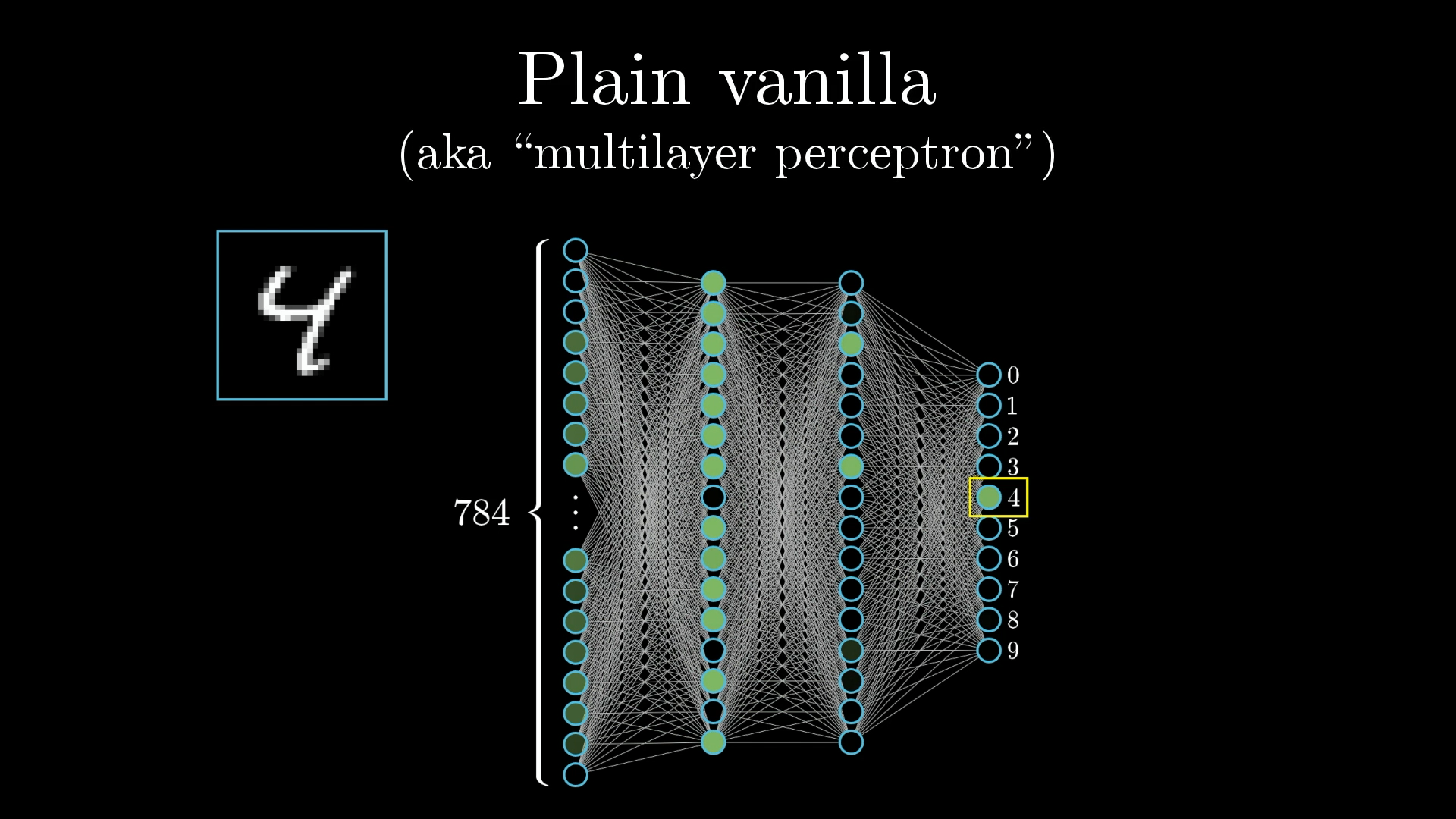
The simple network we’re using to identify digits is just a few layers of neurons linked together.
Neurons
Right now, when I say neuron, all I want you to think is “a thing that holds a number.” Specifically, a number between 0.0 and 1.0. Neural networks are really just a bunch of neurons connected together.
This number inside the neuron is called the “activation” of that neuron, and the image you might have in your mind is that each neuron is lit up when its activation is a high number.
Every neuron has an activation between 0.0 and 1.0, sort of analogous to how neurons in the brain can be active or inactive.
All the information passing through our neural network is stored in these neurons. So we need to represent the inputs and outputs of our network (the images and digit predictions) in terms of these neuron values between 0.0 and 1.0.
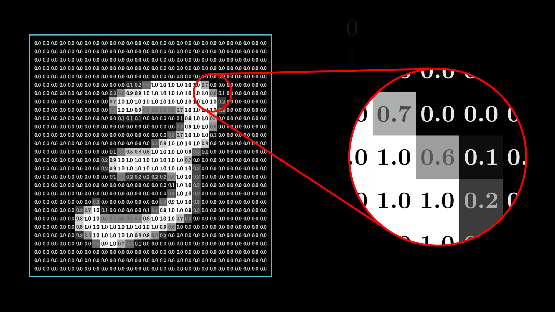
Each pixel in the original image has a value between 0.0 (black) and 1.0 (white).
All of our digit images have pixels, each with a brightness value between 0.0 (black) and 1.0 (white). To represent this in the network, we’ll create a layer of 784 neurons, where each neuron corresponds to a particular pixel.
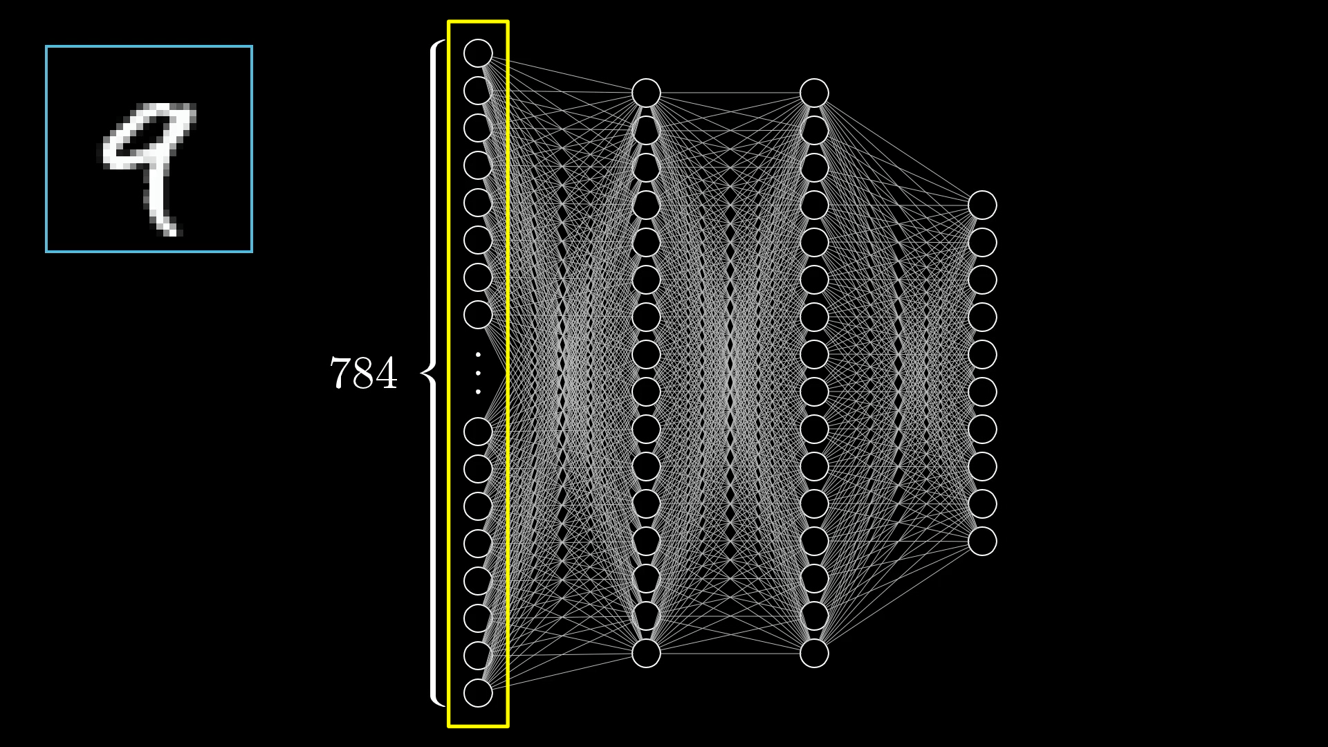
The input layer contains 784 neurons, each of which corresponds to a single pixel in the original image.
When we want to feed the network an image, we’ll set each input neuron’s activation to the brightness of its corresponding pixel.
The last layer of our network will have 10 neurons, each representing one of the possible digits. The activation in these neurons, again some number between 0.0 and 1.0, will represent how much the system thinks an image corresponds to a given digit.
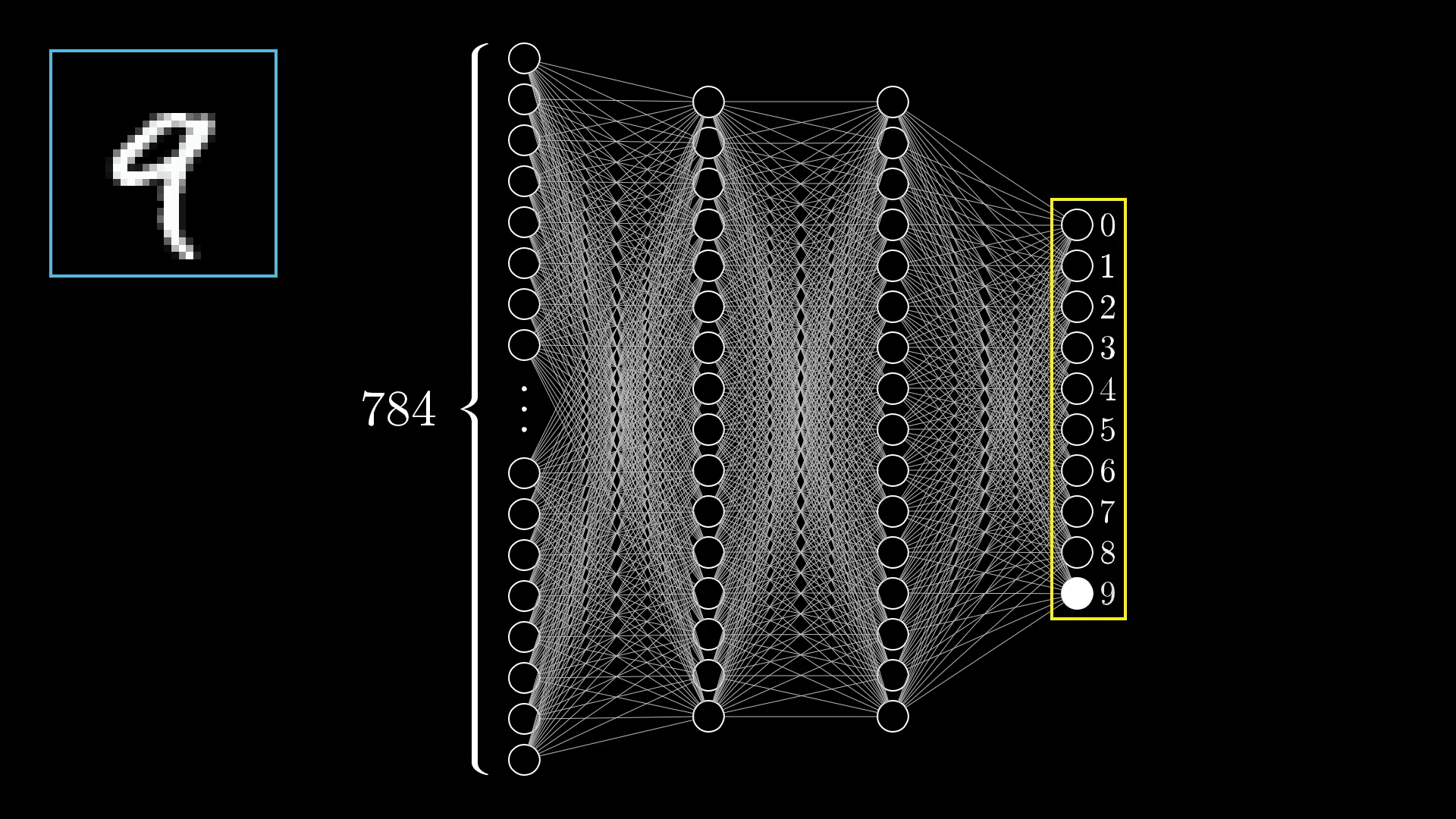
The output layer of our network has 10 neurons. Each neuron corresponds to a particular digit that the image could contain.
Take a look at the following image:
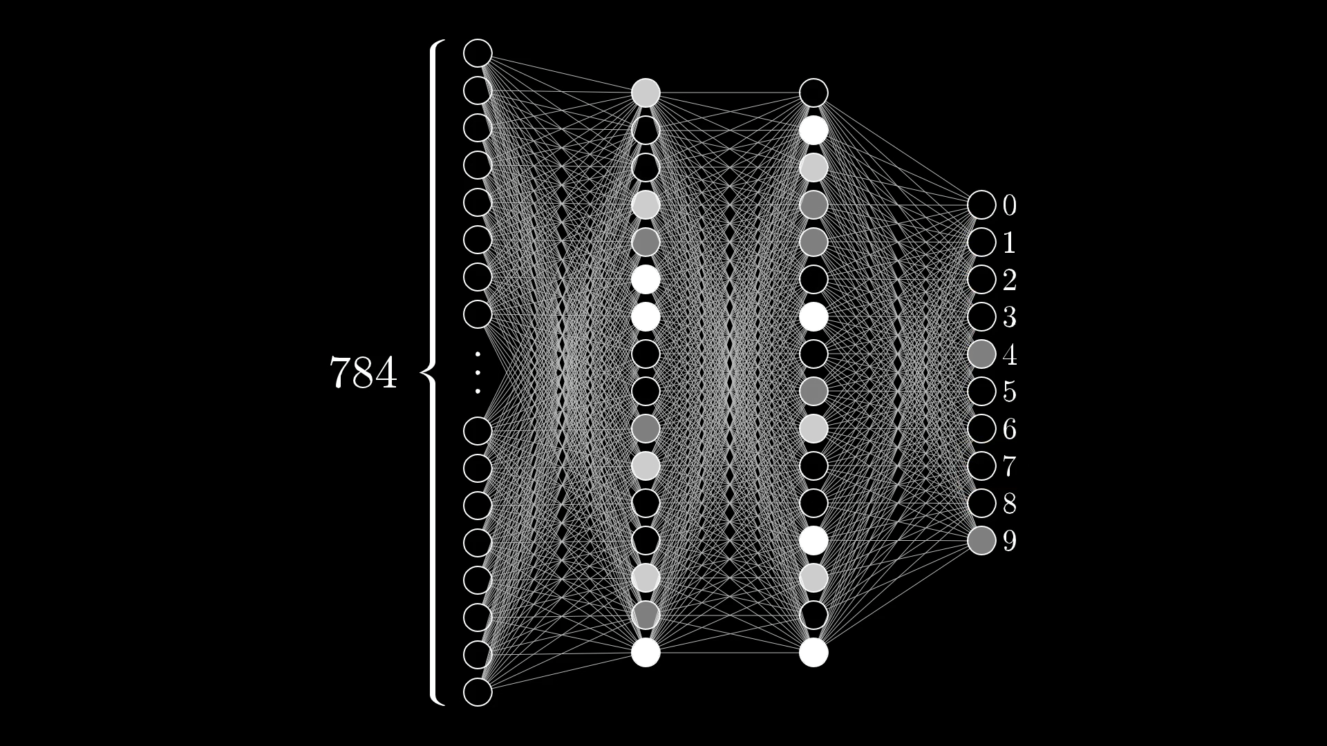
Based on the output layer of the network shown above, what kind of digit does this network think it’s looking at? How certain does it feel?
It’s having trouble deciding whether the input image is a 4 or a 9.
The Hidden Layers
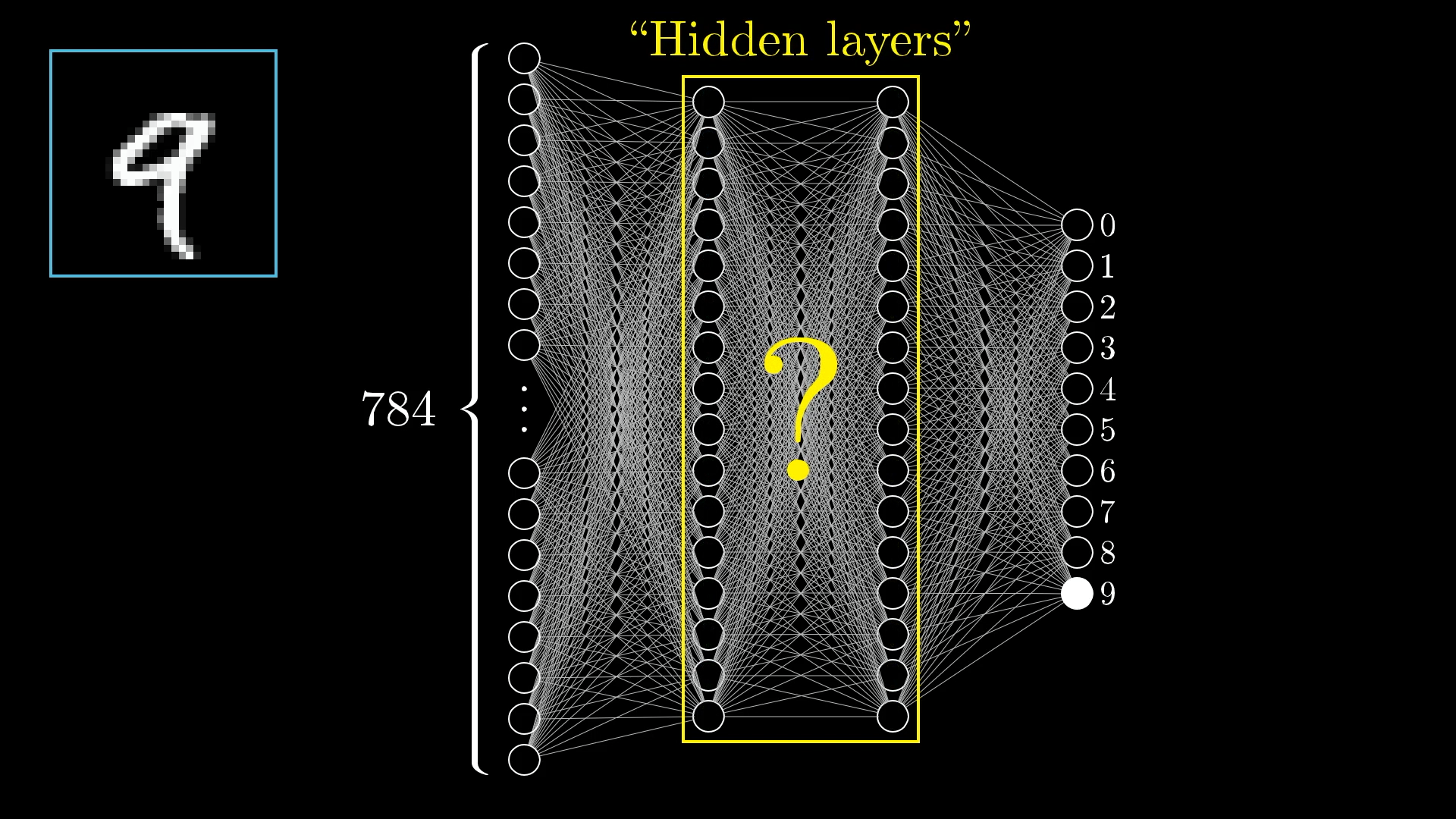
There will also be some layers in between, called “hidden layers”, which for the time being should just be a giant question mark for how on earth this process of recognizing digits will be handled.
In this network I have 2 hidden layers, each with 16 neurons, which is admittedly kind of an arbitrary choice. To be honest, I chose 2 layers based on how I want to motivate the structure in just a moment, and 16 was simply a nice number to fit on the screen. In practice, there’s a lot of room to experiment with the specific structure.
Why Use Layers?
You’ll notice how in these drawings each neuron from one layer is connected to each neuron of the next with a little line. This is meant to indicate how the activation of each neuron in one layer, the little number inside it, has some influence on the activation of each neuron in the next layer.
Watching the activations in each layer propagate through to determine the activations in the next can be quite mesmerizing.
However, not all these connections are equal. Some will be stronger than others, and as you’ll see shortly, determining how strong these connections are is really the heart of how a neural network operates, as an information processing mechanism.
But before jumping into the math for how one layer influences the next, or how training works, let’s talk about why it’s even reasonable to expect a layered structure like this to behave intelligently. What are we expecting here? What’s the best hope for what those middle layers are doing? Why not just directly connect all the pixels to the final output we want?
Well, when you or I recognize digits, we piece together various components like loops and lines.
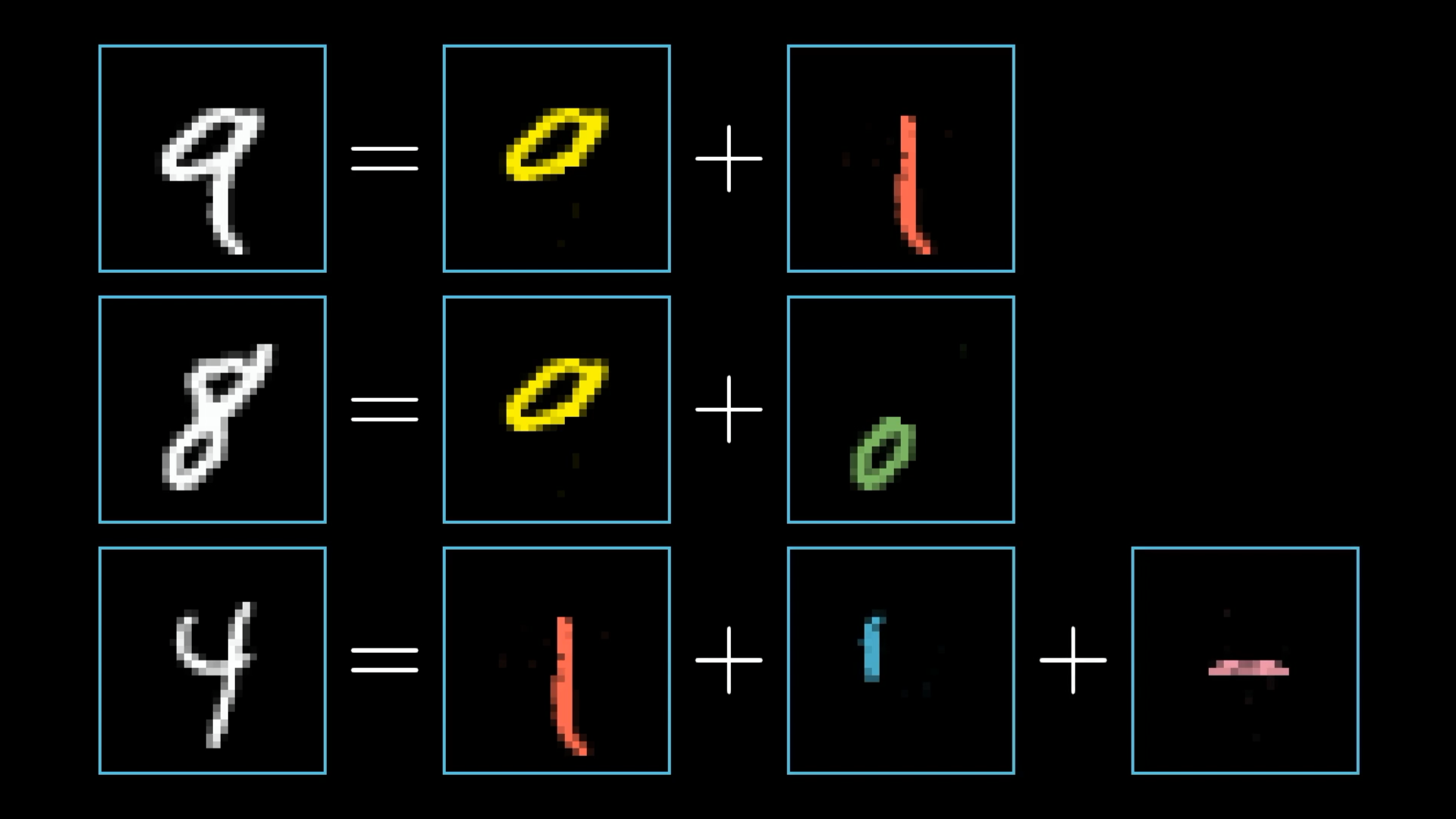
Each digit can be broken into smaller, recognizable subcomponents.
In a perfect world, we might hope that each neuron in the second-to-last layer corresponds to one of these subcomponents. That anytime you feed in an image with, say, a loop up top, there is some specific neuron whose activation will be close to 1.0.
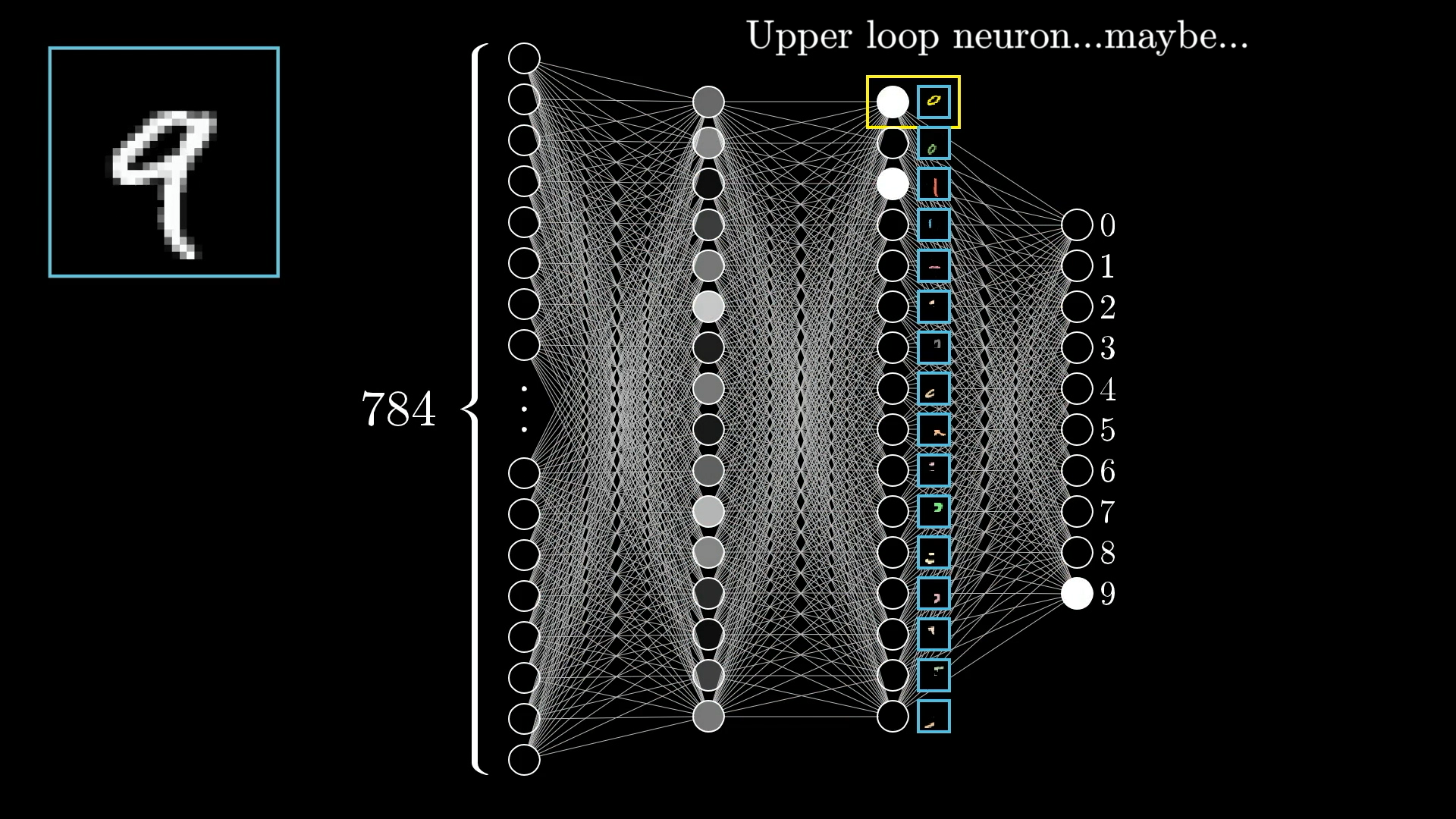
And I don’t mean just this exact loop of pixels. The hope would be that any generally loopy pattern toward the top of the image sets off this neuron. That way, going from this third layer to the last one would only require learning which combinations of subcomponents correspond to which digits.
Of course, this just kicks the problem down the road, because how would you recognize these subcomponents, or even learn what the right subcomponents should be? And I still haven’t talked about how exactly one layer influences the next! But run with me on this for a moment.
Recognizing a loop can also break down into subproblems. One reasonable way to do that would be to first recognize the various edges that make it up.

A loop can be broken down into several small edges.
Similarly, a long line, as you might see in the digits 1, 4 or 7, is really just a long edge. Or maybe you think of it as a certain pattern of several smaller edges.

A long line is also just a bunch of edges.
So our hope might be that each neuron in the second layer of the network corresponds to some little edge. Maybe when an image comes in, it lights up neurons associated with all the specific little edges inside that image. This, in turn, would light up the neurons in the third layer associated with larger scale patterns like loops and long lines, which would then cause some neuron from the final layer to fire which corresponds to the appropriate digit.
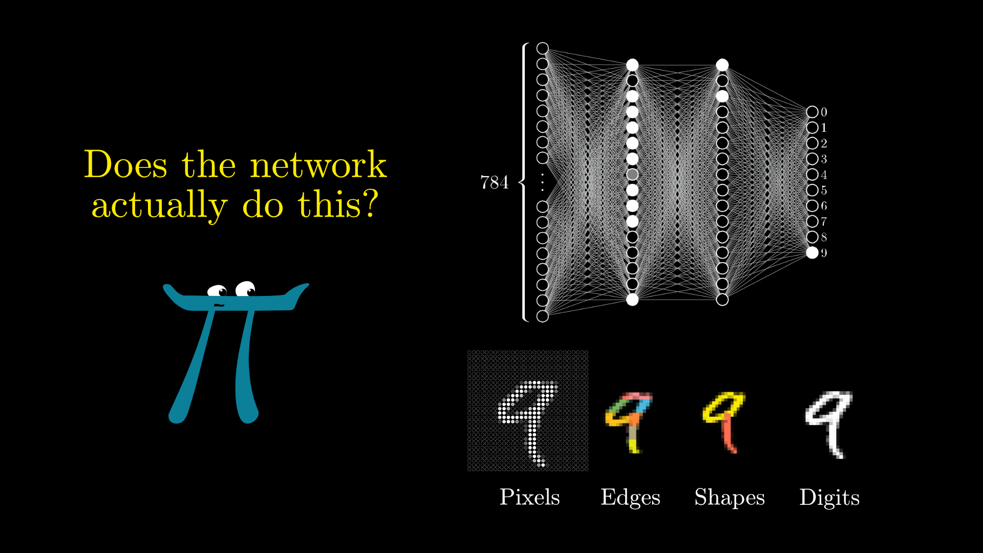
Whether or not this is how our final network actually works is another question. (One that we’ll revisit after seeing how to train this network.) But this is a hope that we might have.
Layers Break Problems Into Bite-Sized Pieces
You can imagine how being able to detect edges and patterns would also be useful for other image-recognition tasks.
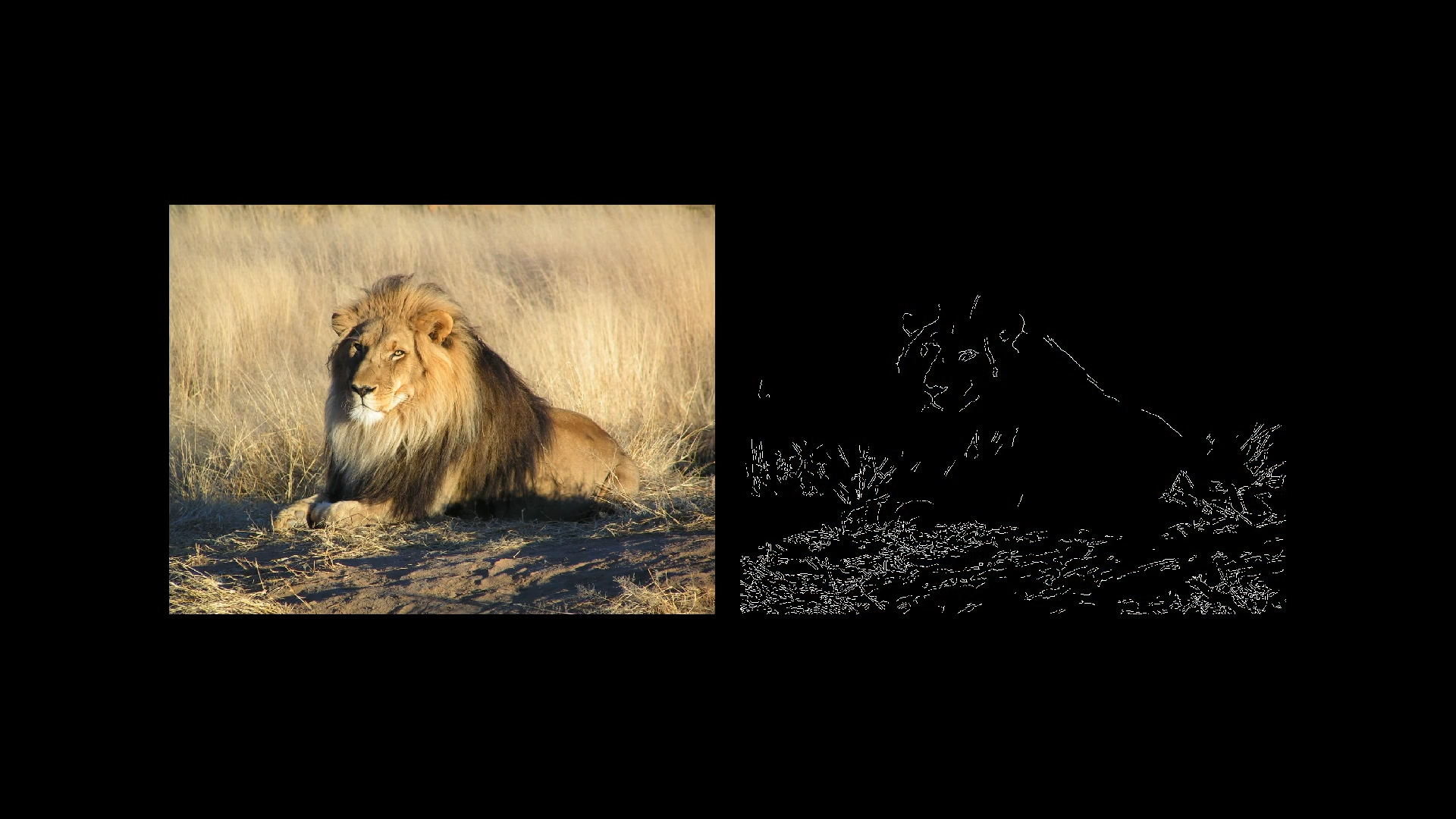
Edge detection isn’t just for digits! It’s a useful step for all kinds of image-recognition problems.
Original lion image by Kevin Pluck, licensed under CC BY 2.0
And beyond image recognition, there are all sorts of intelligent tasks that you can break down into layers of abstraction.
Parsing speech, for example, involves parsing raw audio into distinct sounds, which combine to make certain syllables, which combine to form words, which combine to make up phrases and more abstract thoughts, etc.

The layered structure of the neural network is great because it allows you to break down difficult problems into bite-size steps, so that moving from one layer to the next is relatively straightforward.
How Information Passes Between Layers
With this as a general idea, how do you actually implement it? The goal is to have some mechanism that could conceivably combine pixels into edges, or edges into patterns, or patterns into digits. It would be especially elegant if all of those different steps used the same mathematical procedure.
To zoom in on one very specific example, let’s say that the hope is for this one particular neuron in the second layer to pick up on whether or not the image has an edge in this spot here:
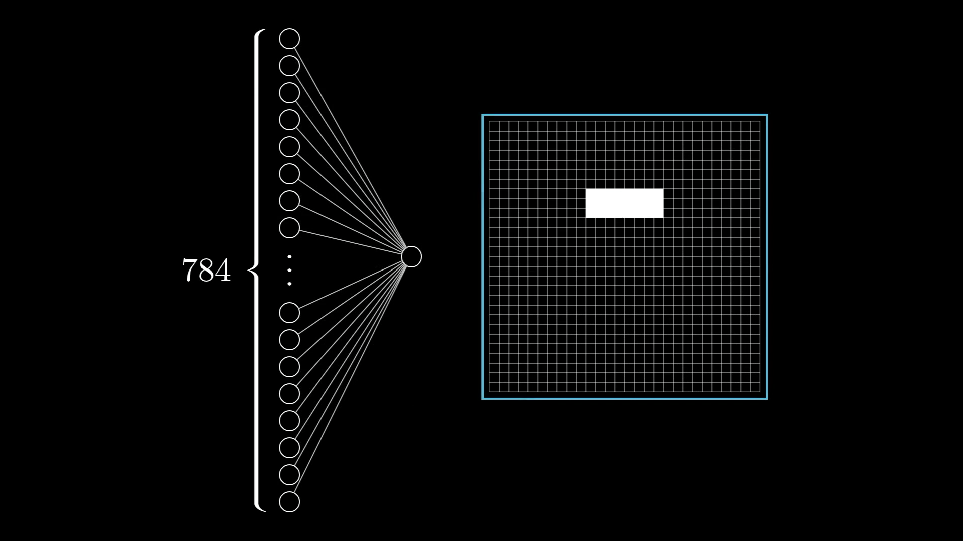
We want this one, specific neuron in the second layer to pick up on whether the image contains this one, specific edge.
I want you to think about what parameters the network should have, what knobs and dials you should be able to tweak, so that it’s expressive enough to potentially capture this pattern. Or other pixel patterns. Or the pattern that several edges can make a loop, and other such things.
What we’ll do is assign a weight to each of the connections between our neuron and the neurons from the first layer. These weights are just numbers.
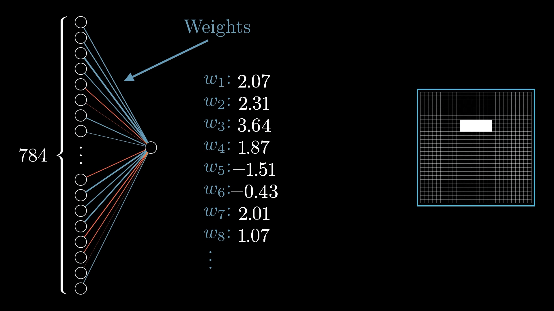
Each weight is an indication of how its neuron in the first layer is correlated with this new neuron in the second layer.
If the neuron in the first layer is on, then a positive weight suggests that the neuron in the second layer should also be on, and a negative weight suggests that the neuron in the second layer should be off.
Of course, these weights will interact and conflict in interesting ways, but the hope is that if we add up all the desires from all the weights, the end result will be a neuron that does a reasonably good job of detecting the edge we’re looking for (as long as the weights are well-chosen).
So to actually compute the value of this second-layer neuron, you take all the activations from the neurons in the first layer, and compute their weighted sum.
It’s helpful to think of all those weights as being organized into a grid of their own:
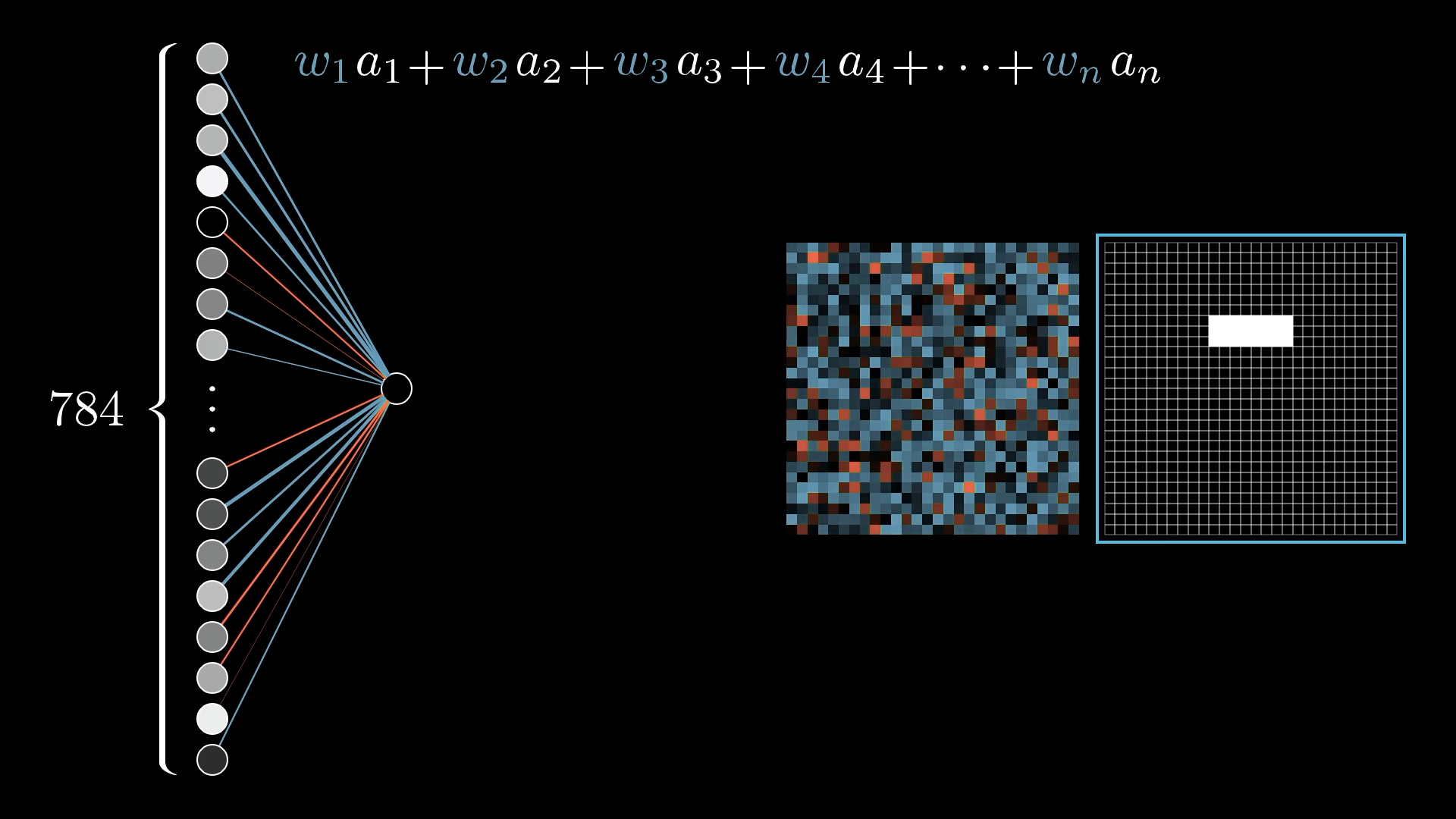
Each weight is associated with one of the 784 input pixels. Arranging the weights into this 28x28 grid makes the correlations between the input image and the output activation clear.
I’m using blue pixels to indicate a positive weight, and red pixels to indicate a negative weight, with the brightness of that pixel being some depiction of the weight’s value.
What if we made the weights associated with almost all the pixels 0, except for some positive weights associated with these pixels in the region where we want to detect an edge?
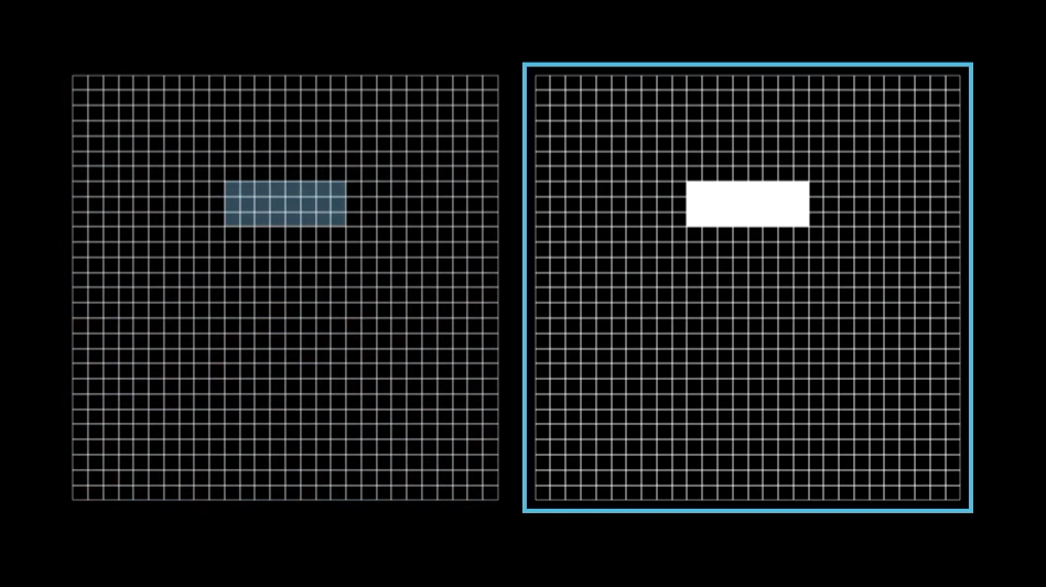
With these weights, the neuron in the second layer will be more activated when pixels in this region are more activated.
Then taking a weighted sum of all pixel values really just amounts to adding up the values of the pixels in this region we care about.
But this pattern of weights will also pick up on big blobs of activated pixels! (Not just edges.) To really pick up on whether or not this is an edge, you might want to have some negative weights associated with the surrounding pixels. Then the sum will be largest when these pixels are bright, but the surrounding pixels are dark.
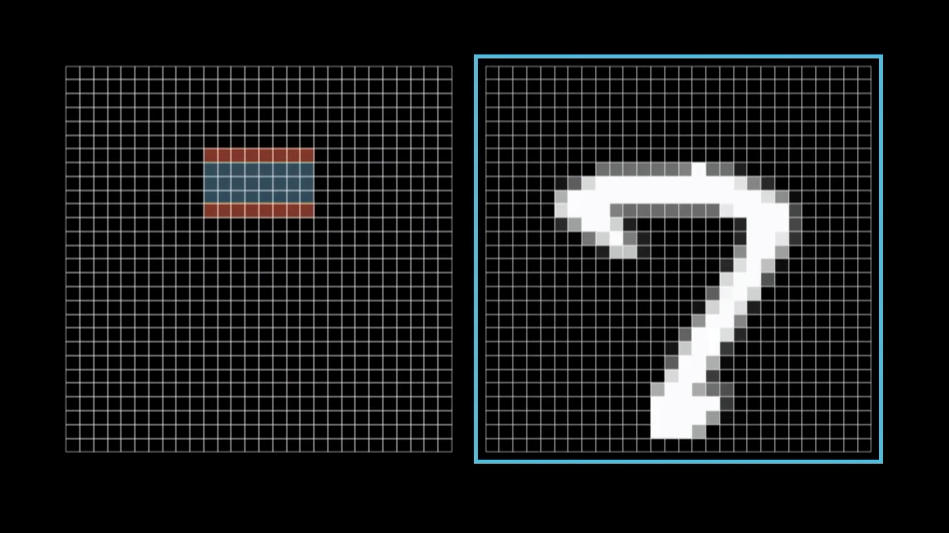
By adding some negative weights above and below, we make sure the neuron is most activated when a narrow edge of pixels is turned on, but the surrounding pixels are dark.
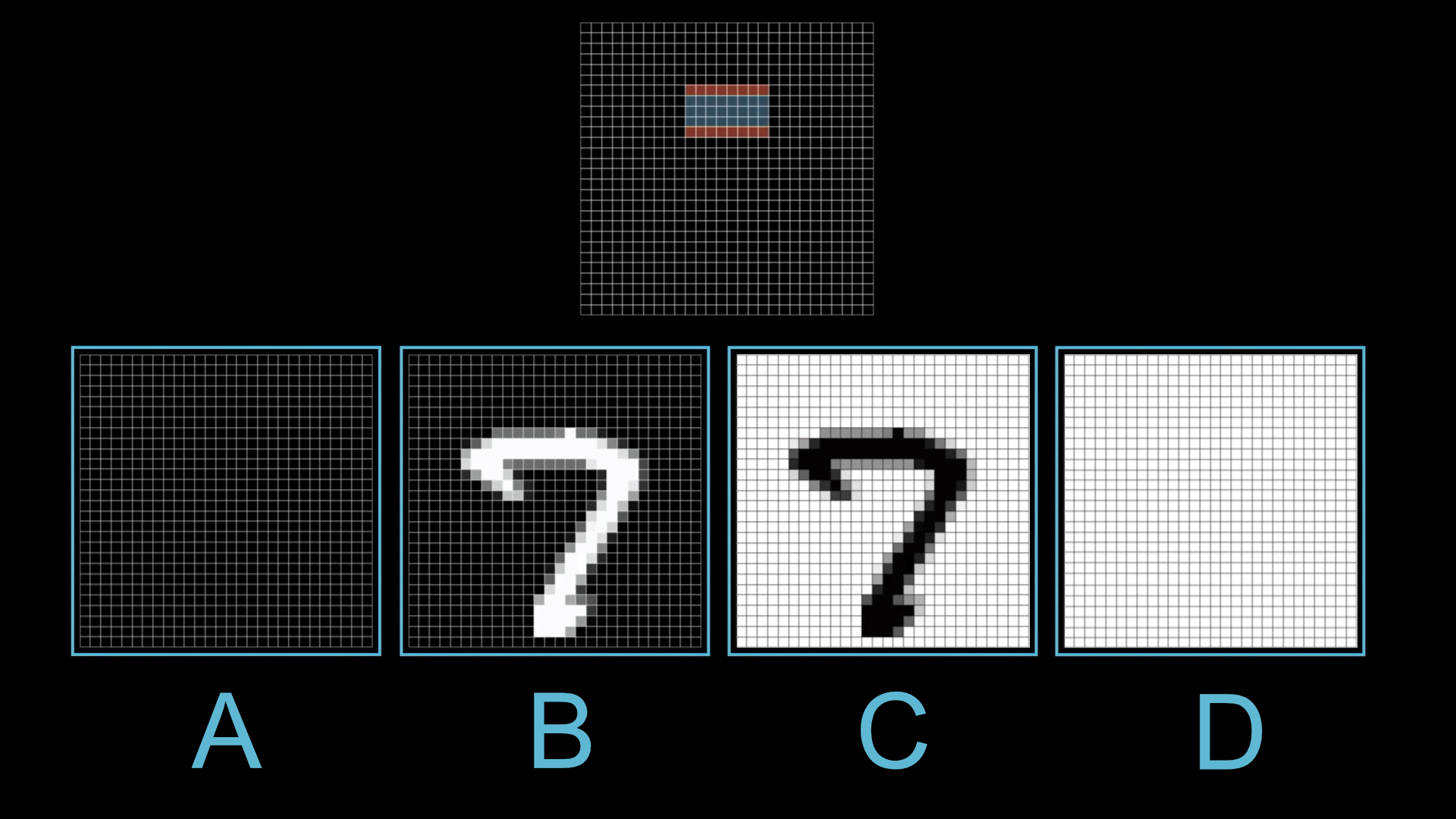
Suppose a neuron in the second layer has weights as indicated above. Rank the four images (A, B, C, and D) based on how much they would activate that neuron:
Sigmoid Squishification
The result of the weighted sum like this can be any number, but for this network we want the activations to be values between 0 and 1. So it’s common to pump this weighted sum into some function that squishes the real number line into the range between 0 and 1.
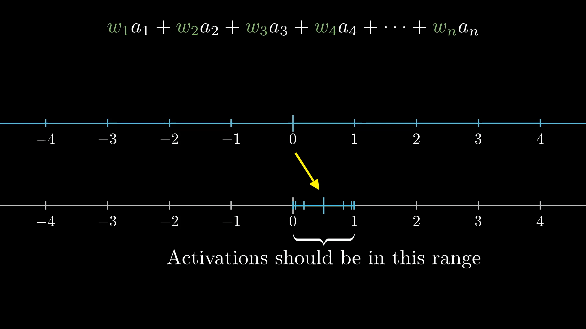
There’s no limit to how big or small the weighted sum might be. But our new neuron value should be between 0 and 1, so we need to somehow squish the range of possible outputs down to size.
One common function that does this is called the “sigmoid” function, also known as a logistic curve, which we represent using the symbol . Very negative inputs end up close to 0, very positive inputs end up close to 1, and it steadily increases around 0. So the activation of the neuron here will basically be a measure of how positive the weighted sum is.
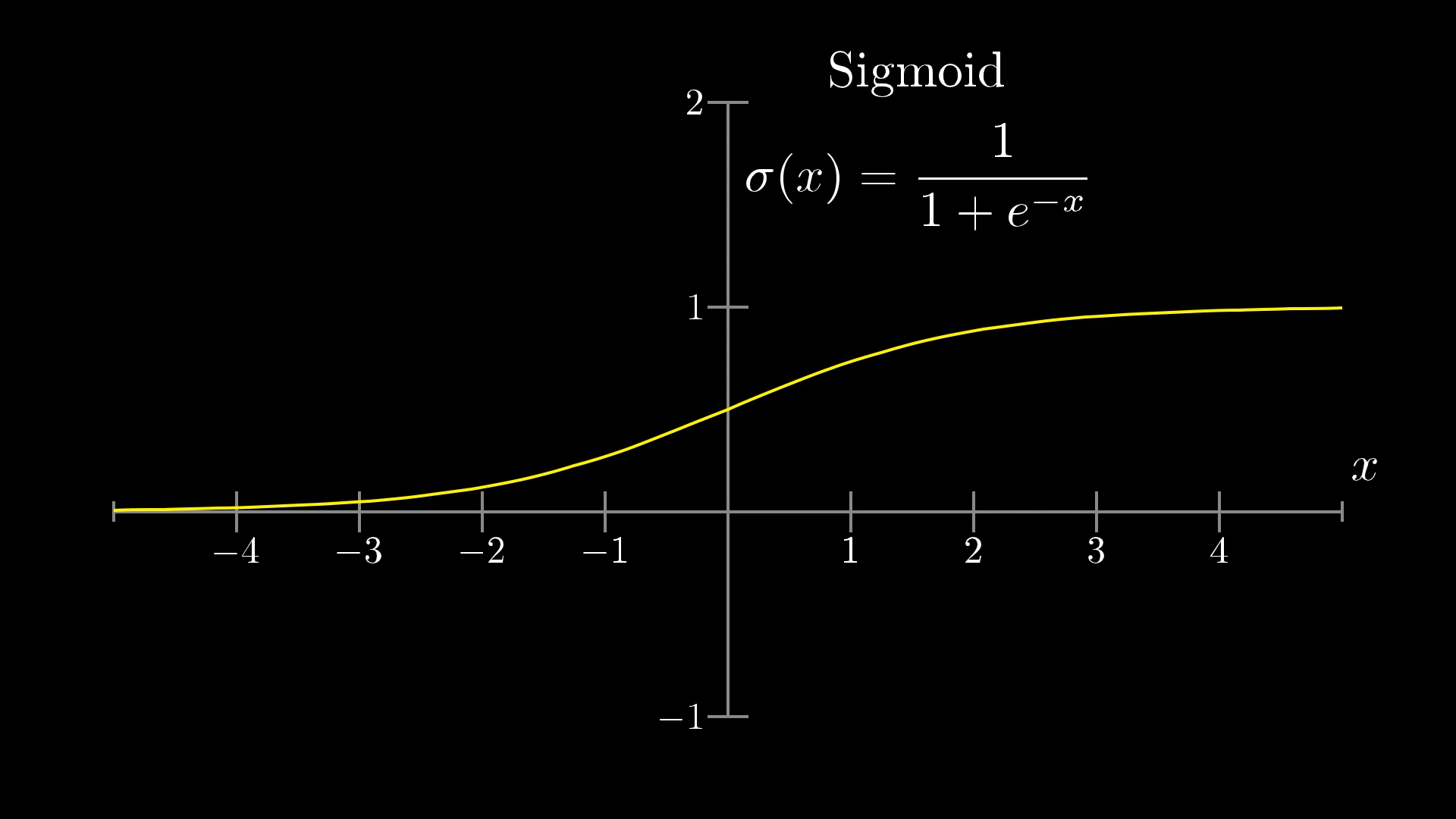
The sigmoid function is just the squishing function we need!
is closest to which of the following values?
But maybe it’s not that we want the neuron to light up when this weighted sum is bigger than 0. Maybe we only want it to be meaningfully active when that sum is bigger than, say, 10. That is, we want some bias for it to be inactive.
What we’ll do then is add some number, like -10, to the weighted sum before plugging it into the sigmoid function that squishes everything into the range between 0 and 1.
We call this additional number a bias.
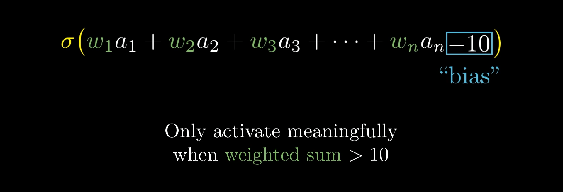
So the weights tell you what pixel pattern this neuron in the second layer is picking up on, and the bias tells you how big that weighted sum needs to be before the neuron gets meaningfully active.
More Neurons
And that’s just one neuron! Every other neuron in the second layer is also going to have weighted connections to all 784 neurons from the first layer. Each neuron also has some bias, some other number to just add on to the weighted sum before squishing it with a sigmoid. That’s a lot to think about! With this hidden layer of 16 neurons, that’s 784x16 weights and 16 biases.
And all of this is just the connection from the first layer to the second. The connections between the other layers also have a bunch of weights and biases as well. All said and done, this network has 13,002 total weights and biases! 13,002 knobs and dials that can be tweaked to make this network behave in different ways.
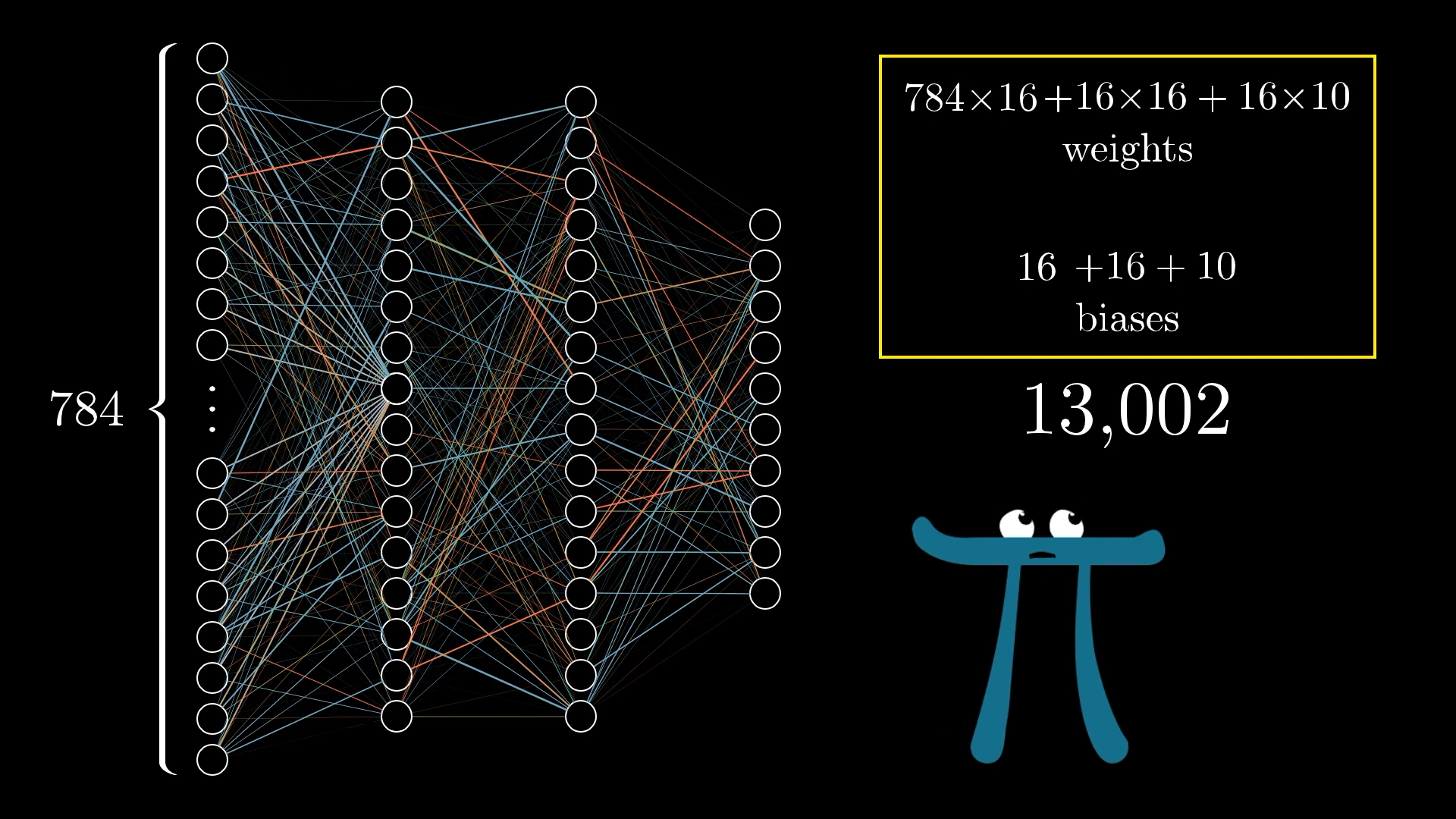
This network has 13,002 weights and biases! That’s a lot to handle.
When we talk about learning, which we’ll do in the next lesson, we mean getting the computer to find an optimal setting for all these many, many numbers that will solve the problem at hand.
One thought experiment, which is at once both fun and horrifying, is to imagine setting all these weights and biases by hand. Purposefully setting weights to make the second layer pick up on edges, the third to pick up on patterns, and so on.
I personally find this satisfying, rather than just treating these networks as a total black box. Because when the network doesn’t perform the way you anticipate, if you’ve built up a feel for the meaning of those weights and biases in your mind, you have a starting place for experimenting with how to change this structure to be better.
Or, when the network does work, but not for the reasons you might expect, digging into what the weights and biases are doing is a good way to challenge your assumptions and really expose the full space of possible solutions.
More Compact Notation
The actual function to get one neuron’s activation in terms of the activations in the previous layer is a bit cumbersome to write down.
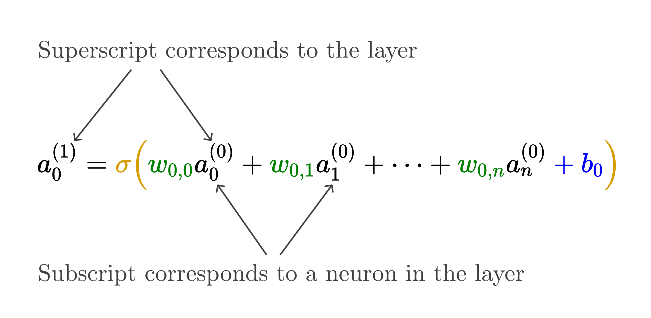
Tracking all these indices takes a lot of effort, so let me show the more notationally compact way that these connections are represented.
Instead of computing a bunch of weighted sums like this one-by-one, we’ll use matrix multiplication to compute the activations of all the neurons in the next layer simultaneously.
First, organize all the activations from the first layer into a column vector.
Next, organize all the weights as a matrix, where each row of this matrix corresponds to all the connections between neurons in the first layer and a particular neuron in the next layer.
Then the product is a column vector containing all the weighted sums for the neurons in the next layer.
Instead of talking about adding the bias to each one of these values independently, we represent it by organizing all those biases into a vector, and adding the entire vector to the previous matrix-vector product:
Finally, I’ll wrap a sigmoid on the outside here, which is meant to represent applying the sigmoid function to each component of the result:
So, once you write this weight matrix and these vectors as their own symbols, you can communicate the full transition of activations from one layer to the next in a neat little expression:
This tiny expression represents the computation of all the neurons in the next layer based on all the neurons in the previous layer, using the chosen weights and biases.
This makes the relevant code much cleaner and much faster, since many libraries optimize the heck out of matrix multiplication.
The Network Is Just a Function
Earlier I said to think of these neurons simply as “things that hold numbers”. Of course, the specific number these neurons hold depends on the image you feed in. So it’s actually more accurate to think of each neuron as a function. It takes in the activations of all neurons in the previous layer, and spits out a number between 0 and 1.
And really, the entire network is just a function! It takes in 784 numbers as its input, and spits out 10 numbers as its output. It’s an absurdly complicated function, because it takes over 13,000 parameters (weights and biases), and it involves iterating many matrix-vector products and sigmoid squishificaitons together. But it’s just a function nonetheless.
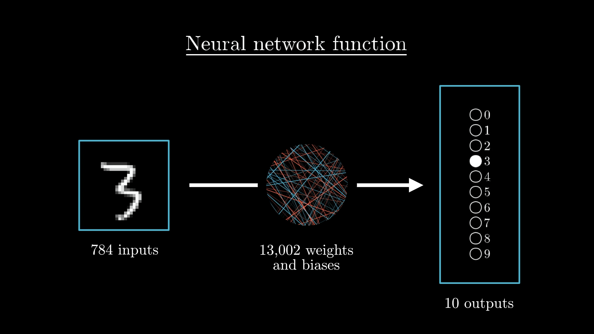
The entire neural network is a function that uses all its weights and biases to take in 784 input pixels and spit out 10 output numbers.
Next up: Learning!
In a way, it’s kind of reassuring that this looks complicated. If it were any simpler, what hope would we have that it could take on the challenging task of recognizing digits?
And how does it take on that challenge? How does this network learn the appropriate weights and biases from data? That’s what I’ll show in the next lesson.
Oh, but before you go, I do have one little asterisk to mention about the sigmoid function if that sounds interesting to you:
Thanks
Special thanks to those below for supporting the original video behind this post, and to current patrons for funding ongoing projects. If you find these lessons valuable, consider joining.