Chapter 16The other way to visualize derivatives
Introduction

Picture yourself as a calculus student, about to begin your first course. The months ahead of you hold within them a lot of hard work, neat examples, not-so-neat examples, beautiful connections to physics, not-so-beautiful piles of formulas to memorize, plenty of moments getting stuck and banging your head into a wall, a few “aha” moments sprinkled in as well, and some truly lovely graphical intuitions to help guide you throughout it all.

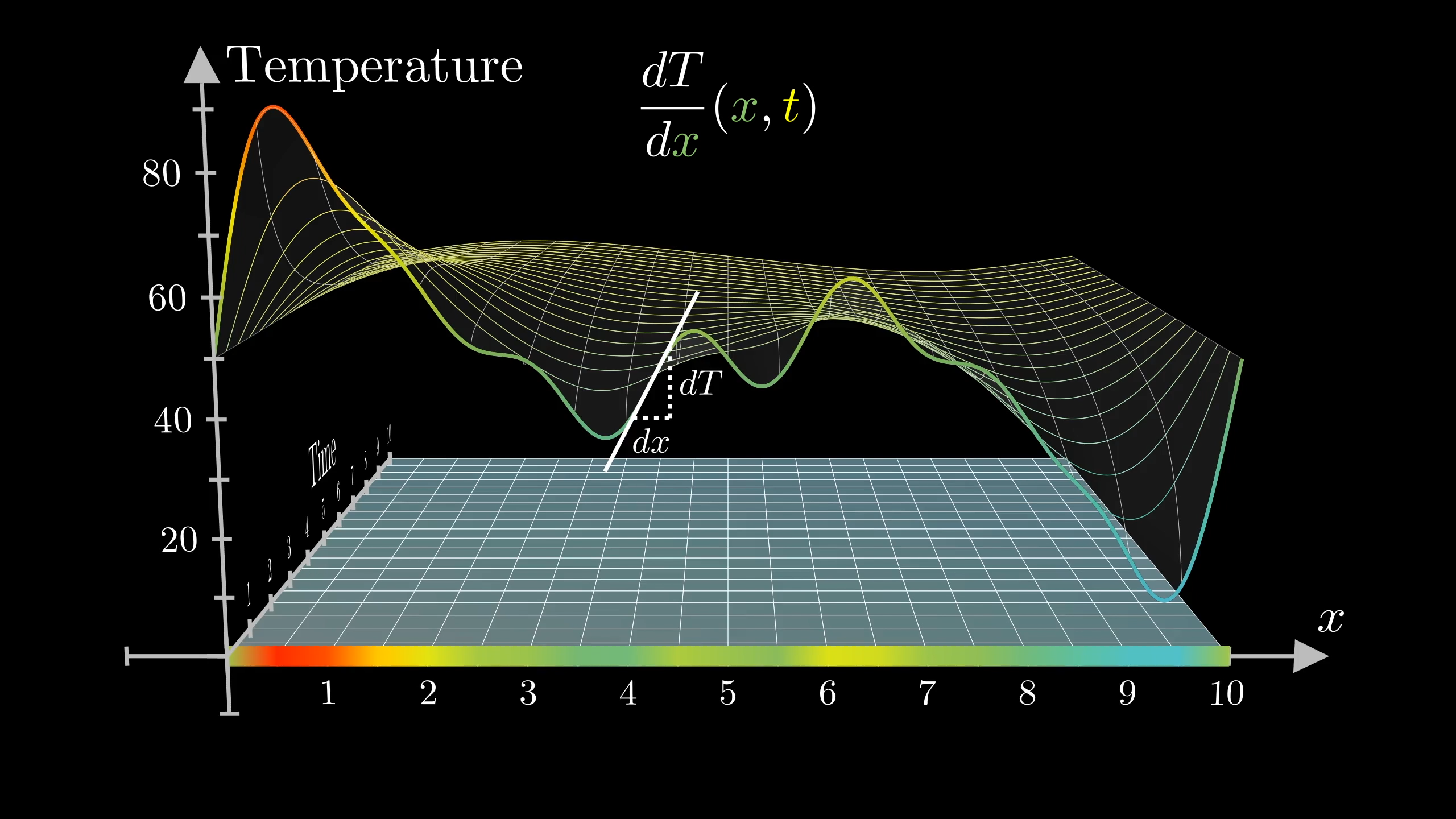
A graphical depiction of a partial differential equation.
But if the course ahead of you is anything like my first introduction to calculus, or any of the first courses I've seen in the years since, there's one topic you will not see, but which I believe stands to greatly accelerate your learning.
You see, almost of all the visual intuitions for a first year in calculus are based on graphs. The derivative is the slope of a graph, the integral is an area under that graph, etc.
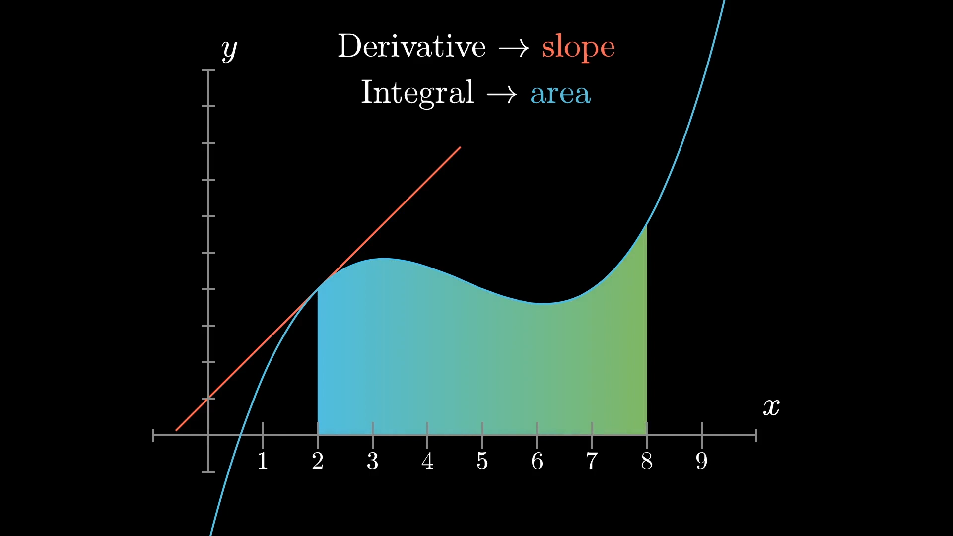
But as you generalize calculus beyond functions whose inputs and output are simply numbers, it's not always possible to graph the function your analyzing.
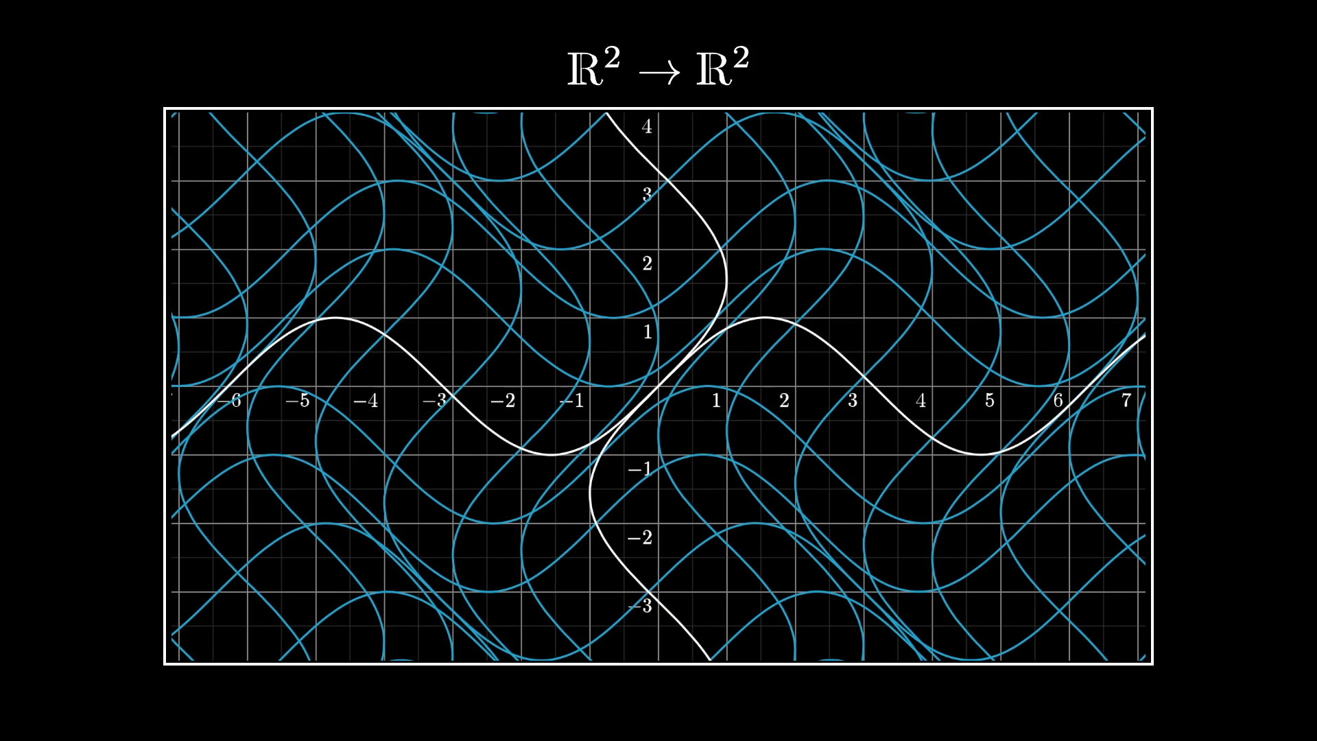
If your intuitions for fundamental ideas like the derivative are rooted too rigidly in graphs, this can make for a very tall and largely unnecessary conceptual hurdle between you and the more “advanced” topics like multivariable calculus, complex analysis, differential geometry, etc.
What I want to share with you is a way of thinking about derivatives, which I'll refer to as the transformational view, which generalizes more seamlessly into some of the more general contexts where calculus shows up. And then we'll use it to analyze a certain fun puzzle about repeated fractions.
The transformation view
First off, let's just make sure we're all on the same page about what the standard visual is. If you graph a function which simply takes real numbers as inputs and outputs, one of the first things you learn in a calculus course is that the derivative gives you the slope of this graph.
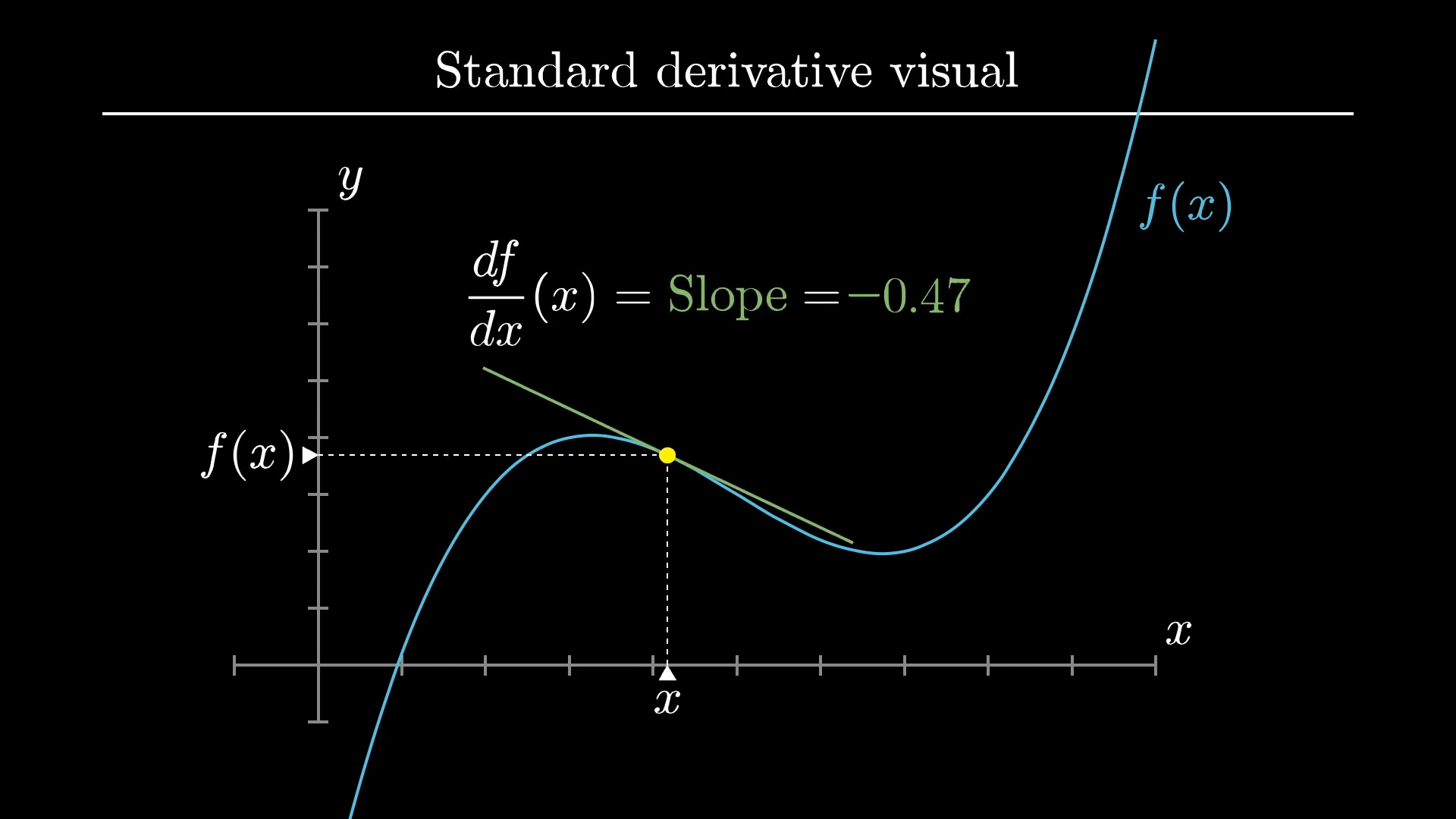
What we mean by that is that the derivative of the function is a new function which for every input x, returns this slope.
Quick sanity check! What's the derivative of ?
I'd encourage you not think of this derivative-as-slope idea as being the definition of the derivative; instead think of the derivative as asking how sensitive is the function to tiny nudges around a given input. The slope of the graph is just one way to think about that sensitivity, relevant only to this particular way of viewing functions.
The basic idea behind the alternate visual for the derivative is to think of the function as mapping all possible inputs on a number line to their corresponding outputs on a different number line.
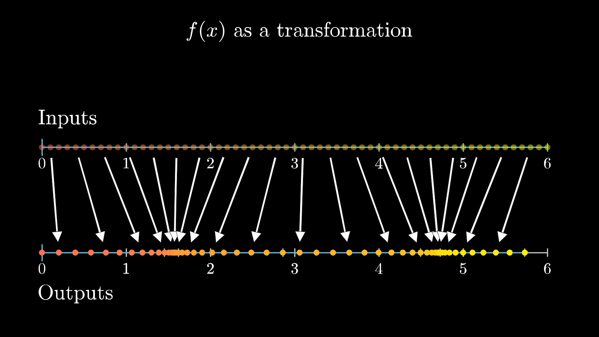
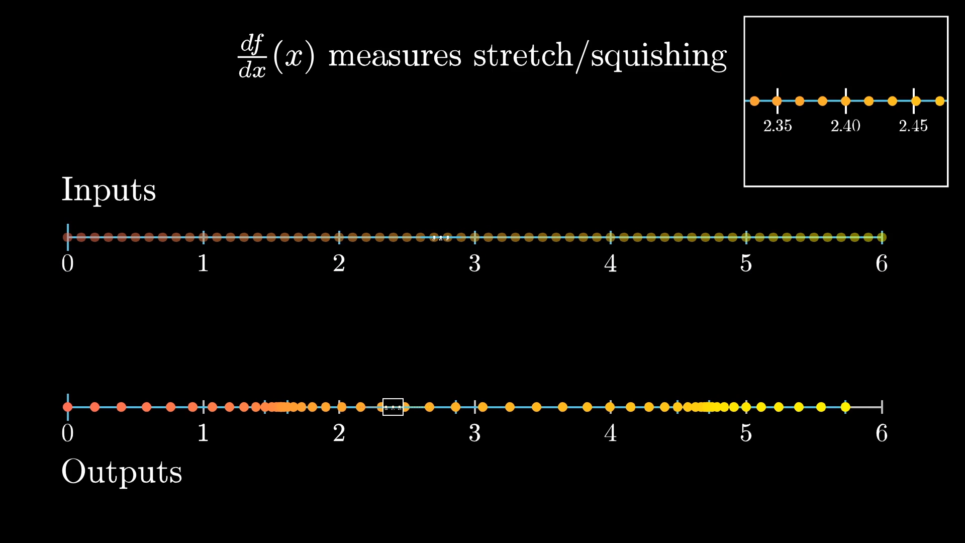
In this case the derivative gives a measure of how much this input space gets stretched or squished in various regions. That is, if you zoom in around some specific input, and look at some evenly spaced points around it, the derivative of the function at that input will tell you how spread out or contracted those points become.
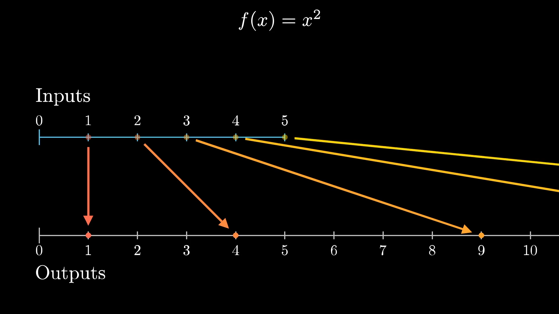
A specific example helps. The function maps the point at to , the point at to , the point at to , and so on.
If you were to zoom in on a little cluster of points around , and see where they land around the relevant output, which for this function happens to also be , you'd notice they get stretched out.
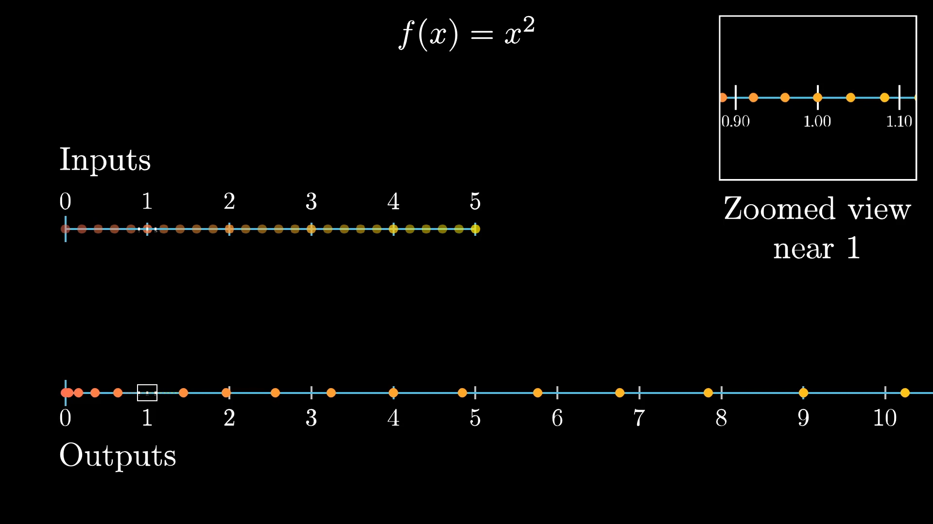
In fact, it roughly looks like stretching out by a factor of . And the closer you zoom in, the more this local behavior just looks like multiplying by a factor of . This is what it means for the derivative of at to be ; it's what that fact looks like in the context of transformations.
If you looked at a neighborhood of points around the input , they would roughly get stretched out by a factor of , which is what it means for the derivative of this function at the input to be .
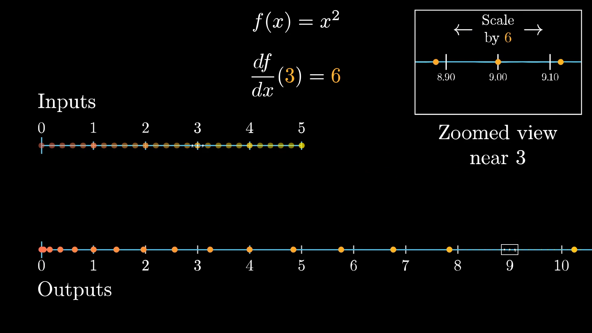
Around the point , what factor would the surrounding points stretch out by?
The input zero is interesting: Zooming in by a factor of , it doesn't exactly look like a constant stretching or squishing.
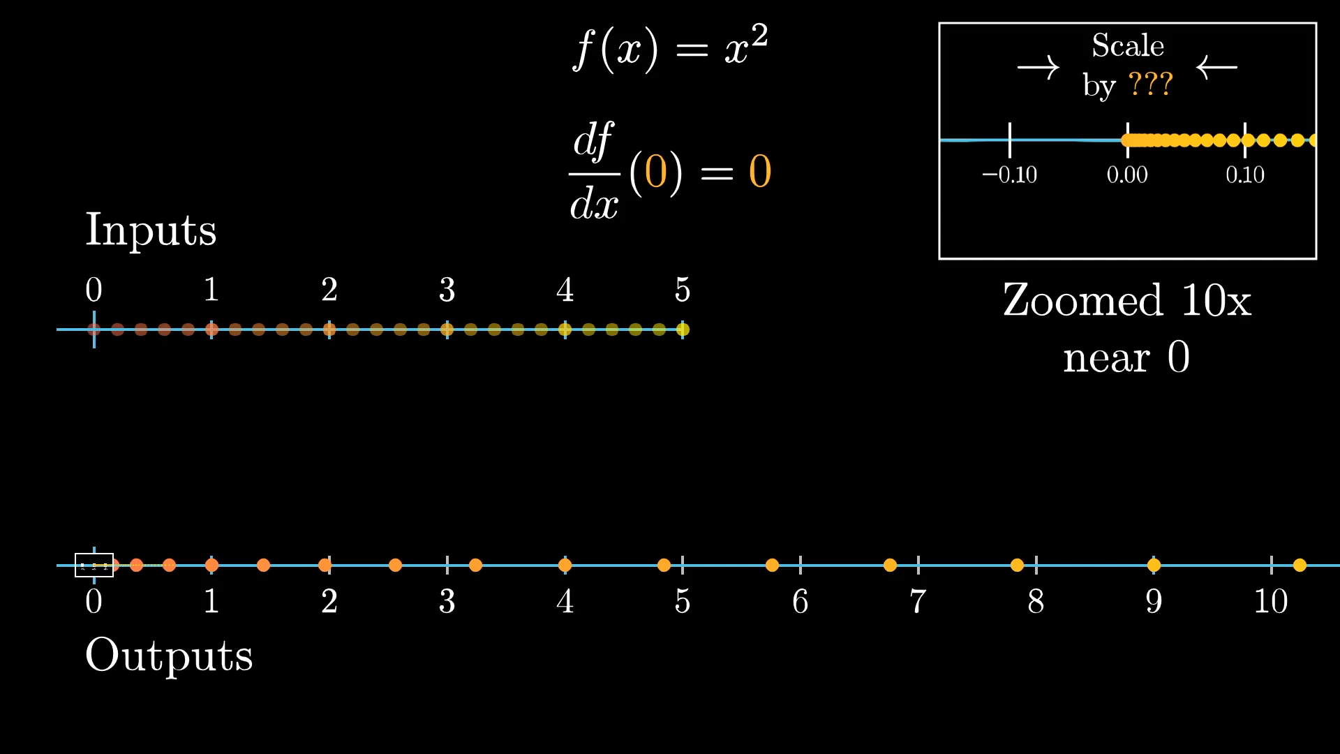
For one thing, all the outputs end up on the right positive side of things. As we zoom in closer, by x, or x, it looks more and more like the small neighborhood around zero gets collapsed to a point.
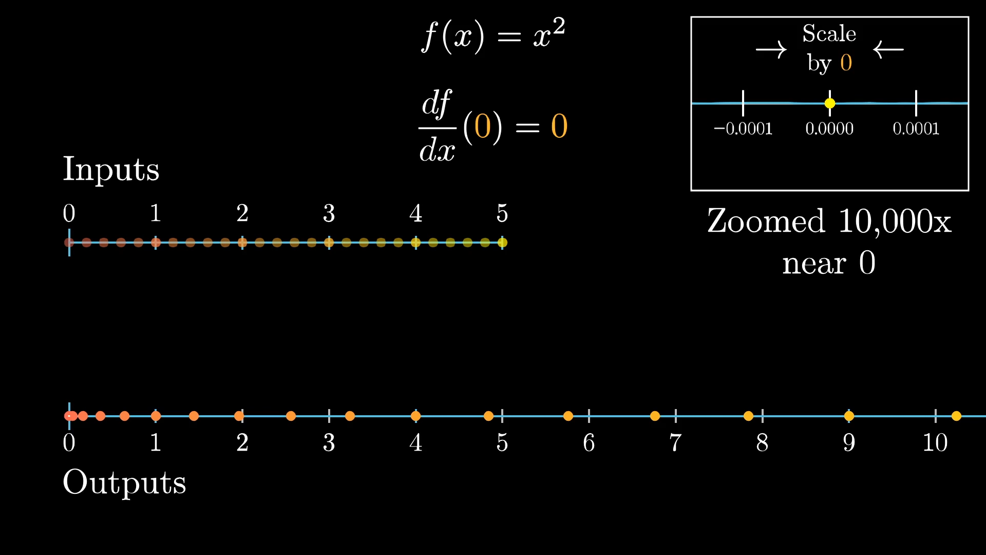
This is what it looks like for a derivative to be , the local behavior looks more and more like multiplying a number line by . It doesn't have to completely collapse things to a point at any particular zoom level; instead it's a matter of what the limiting behavior is here.
If you also considered negative inputs, things start to feel a little cramped, since these collide with all those positive input values. This is one downside of thinking of functions transformations. But for derivatives, we only care about local behavior anyway; that is, what happens in a small range around a given input.
We really only care about local behavior here.

Notice that the inputs in a little neighborhood around, say, , don't just get stretch out, they also get flipped around.
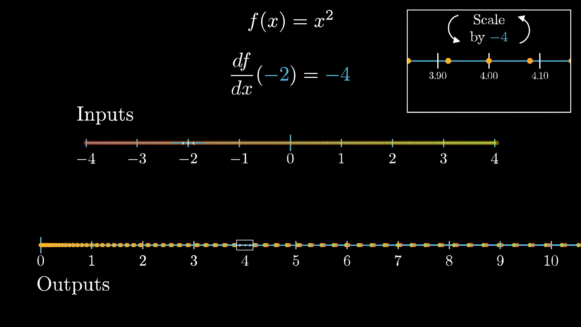
Specifically, the action on such a neighborhood looks more and more like multiplying by the closer you zoom in. This is what it looks like for a function to have a negative derivative.
Given this interpretation of the derivative, can you come up with a formula for it using expressions you're already familiar with?
An application of this derivative view
This is all well and good, but let's see how it's useful in solving a problem.
A friend of mine recently asked me a pretty fun question about this infinite fraction:
Maybe you've seen this before, but my friend's questions cuts to something you may not have thought about before, relevant to the view of the derivative we're looking at here.
A typical way you might evaluate an expression like this is to first set it equal to .
Then, notice that there is a copy of the full fraction inside itself, giving us this:
You can also think of this as finding a fixed point of the function . But here's the thing, there are actually two solutions for ; two special number where plus over that number gives you back the same number.
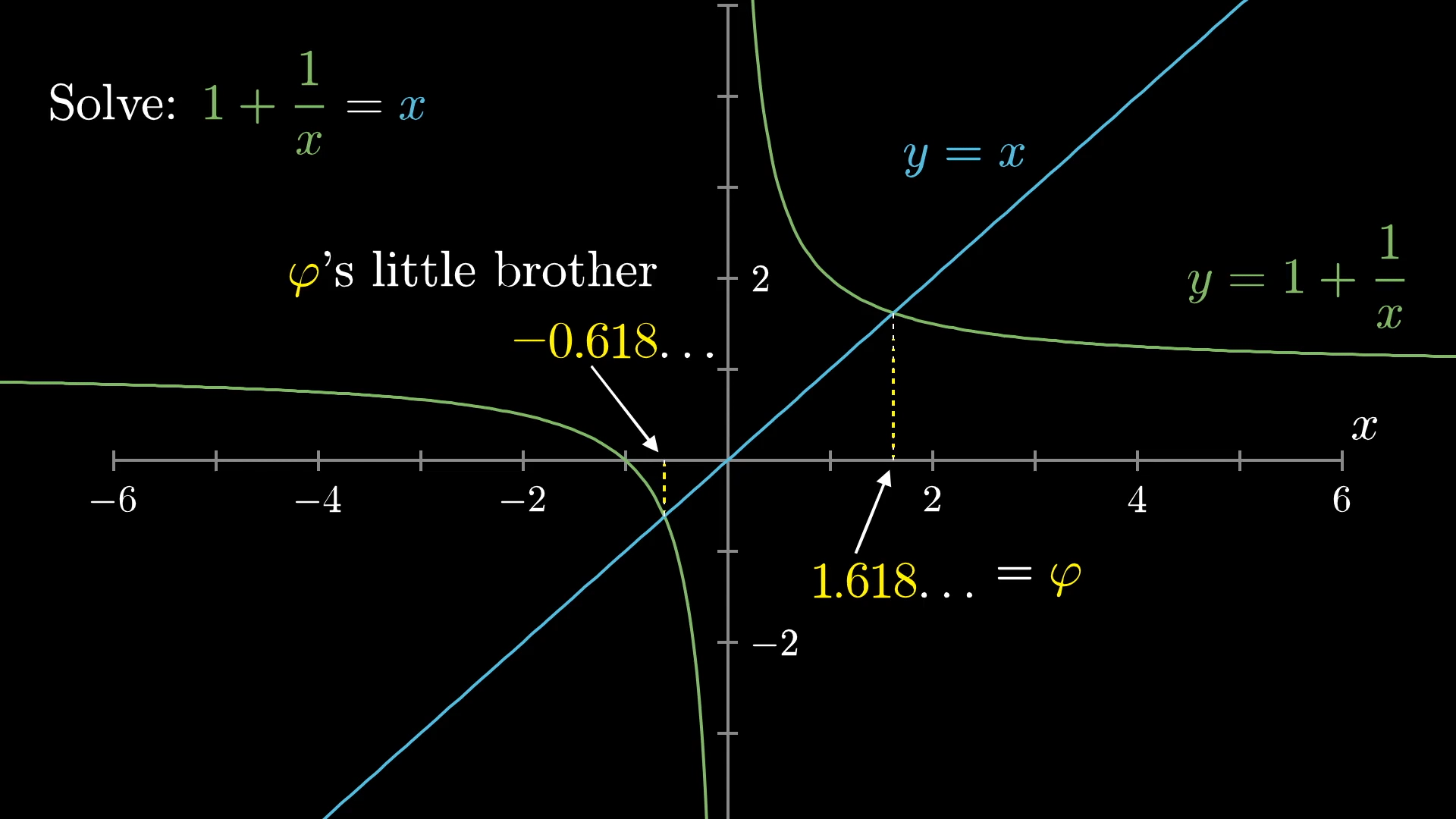
One is the golden ratio , around , and the other is at , which is . I like to call this other number 's "little brother", since just about any property has, this number also has. So would it be valid to say that this infinite fraction also equals 's little brother, ?
Which one is the answer?

Maybe you initially say “obviously not!”. Everything on the left-hand side is positive, so how could it equal a negative number? Well, first let's be clear about what we mean by an expression like this.
One way to think of it, though it's not the only way, is to imagine starting with some constant, like , then repeatedly applying the function , and asking about what this approaches as you keep going.
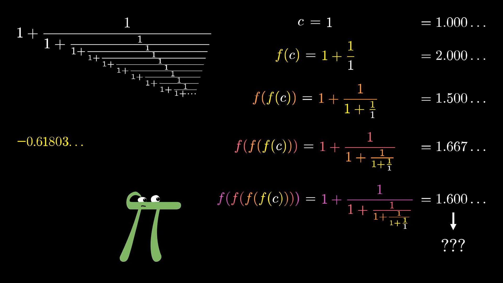
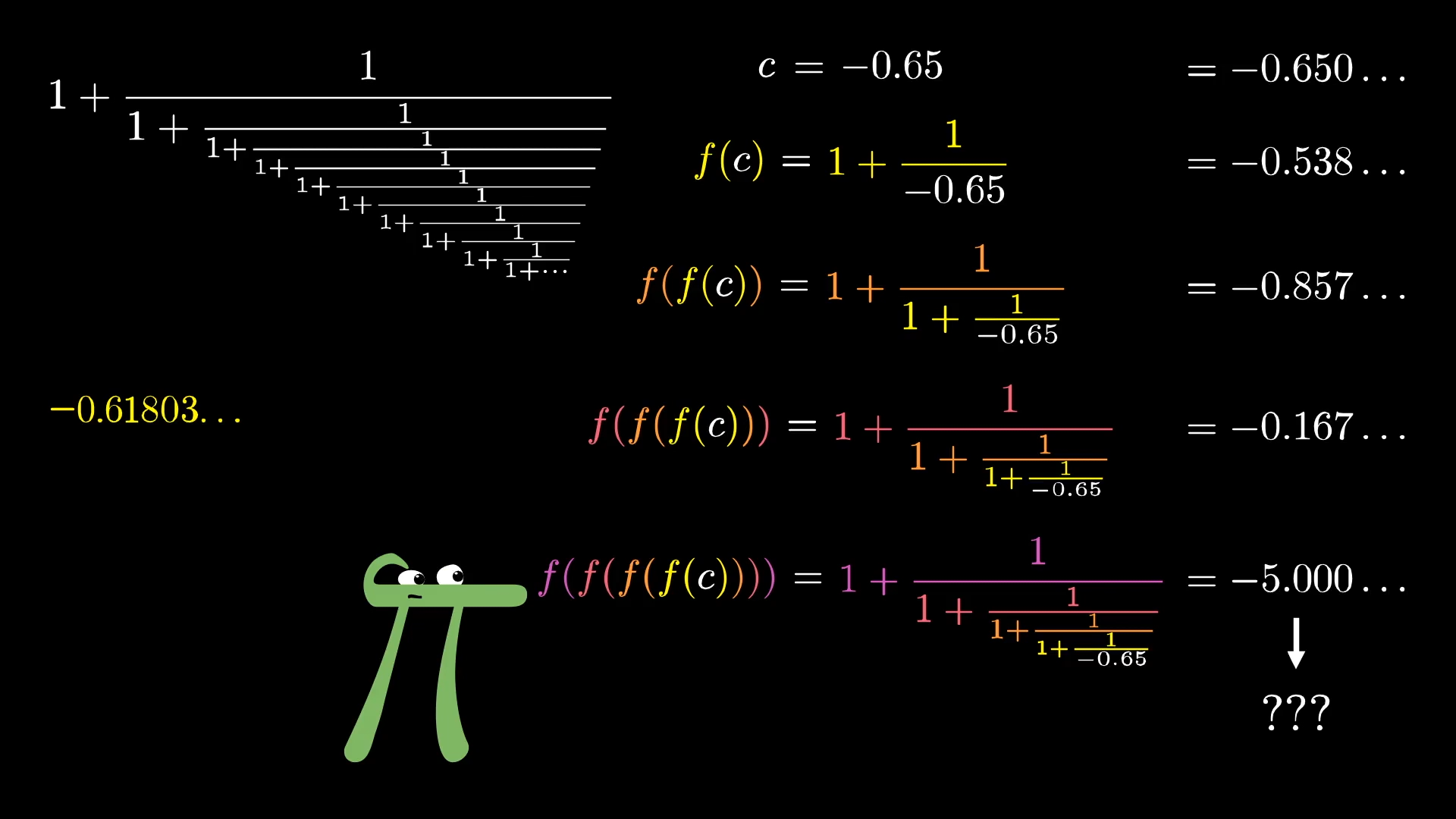
So in that view, maybe if you start with a negative number, it's not so crazy for the whole expression to end up negative.
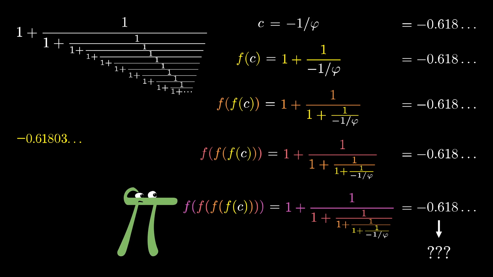
After all, if you start with , then apply the function , you get back . So no matter how many times you apply it, you'll stay fixed at that value.
Well, even then, there is one reason you view as the favorite brother in this pair. Try this, pull up a calculator of some kind, start with any random number, then plug it into this function . Then do it again. And again. And again and again and again.
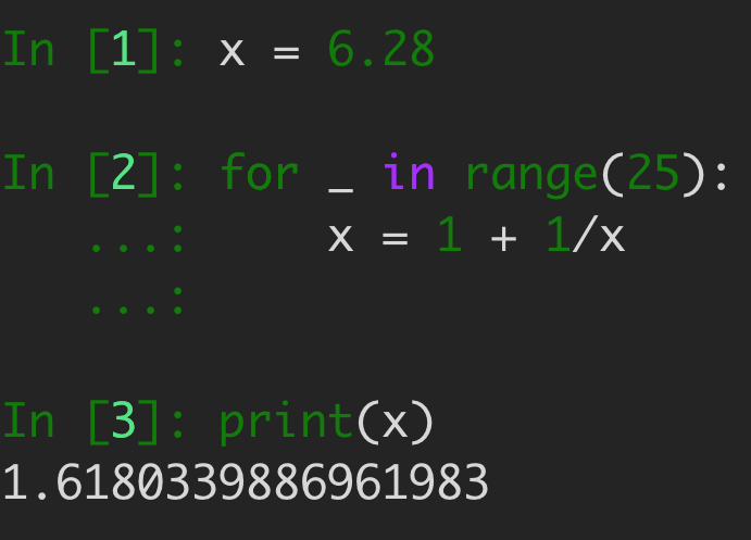
No matter what constant you start with, you will eventually end up at . Even if you start with a negative number, even one really really close 's little brother, eventually it will shy away from that value and jump back to phi.
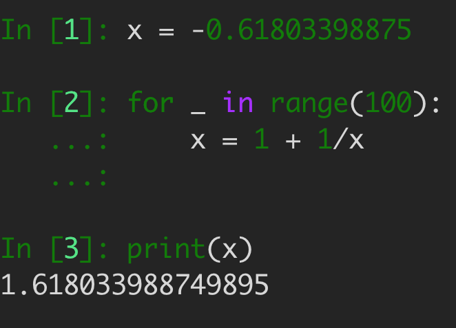
So what's going on here? Why is one of these fixed points favored over the other?
Maybe you can already see how the transformational understanding of derivatives will help us to understand this setup, but for the sake of having a point of contrast, let me show how a problem like this is often taught using graphs.
If you plug in some random input to this function, the -value tells you the corresponding output.
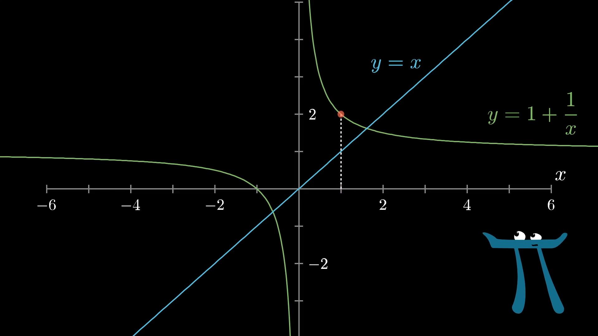
To think about plugging that output back into the function, you might first move horizontally until you hit the line , which will get you to a position where the -value corresponds to your previous output.
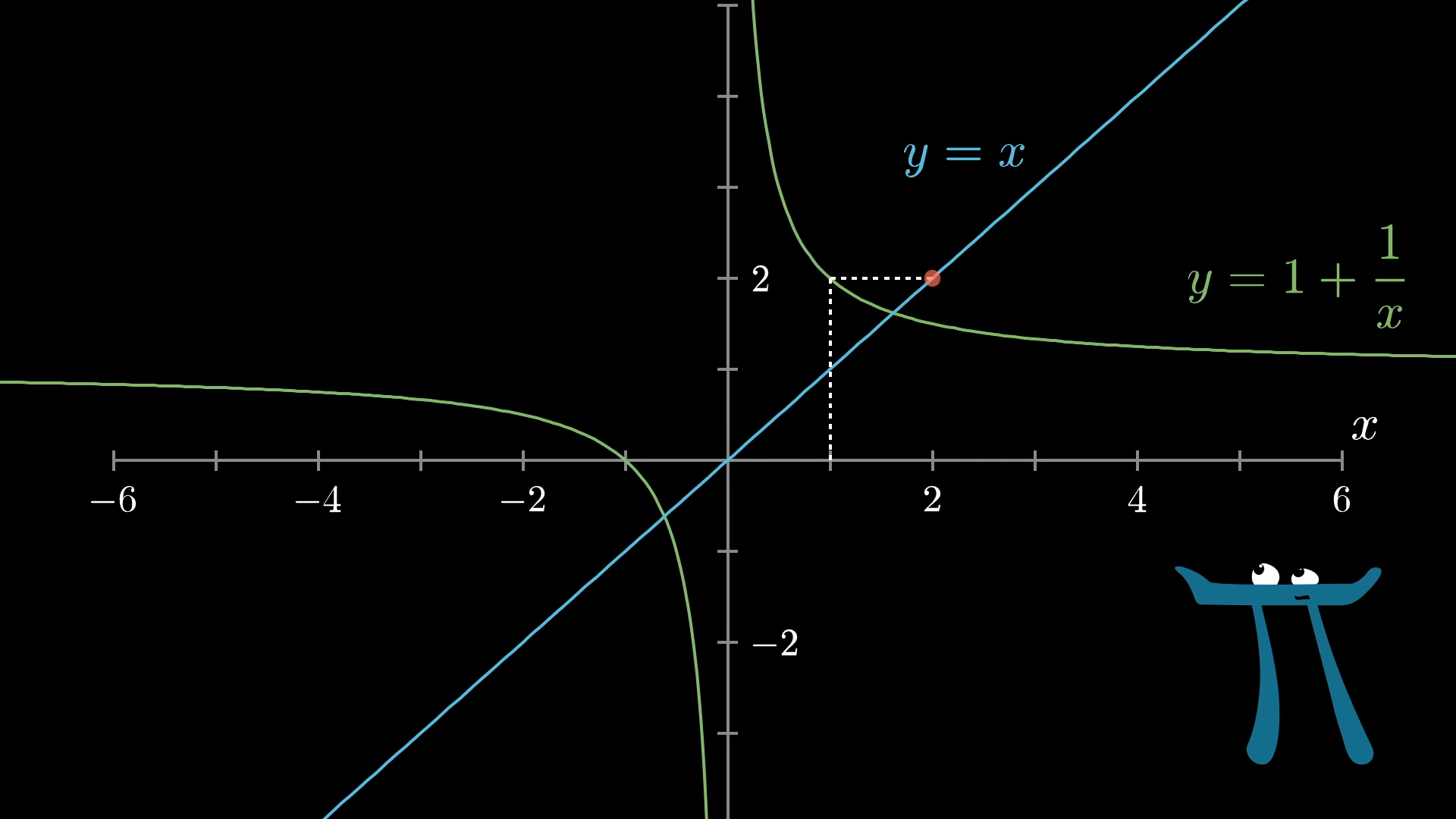
Then, you can move vertically to see what the output at this new -value is.
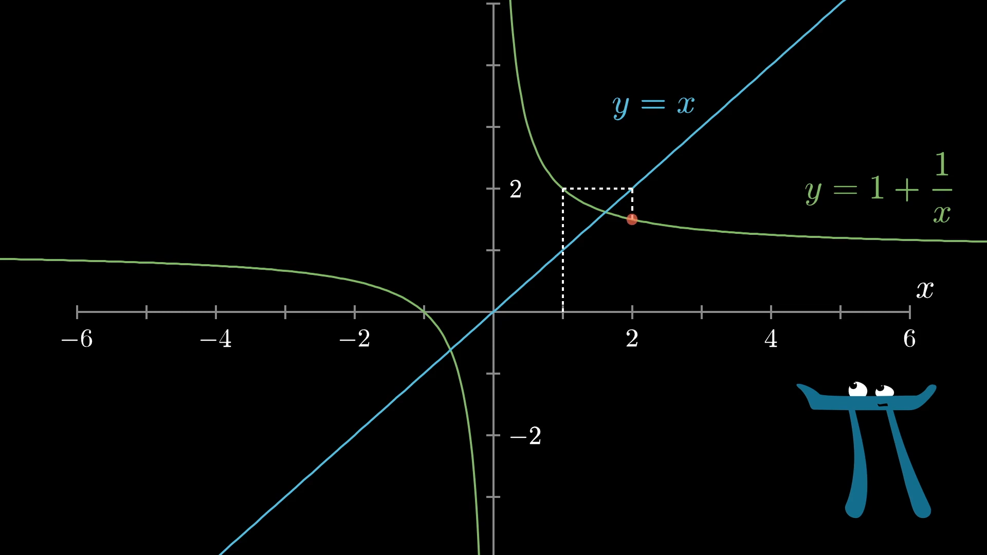
Then repeat: Move horizontally to the line to find a point whose -value is the same as the output you just got, then move vertically to apply the function.
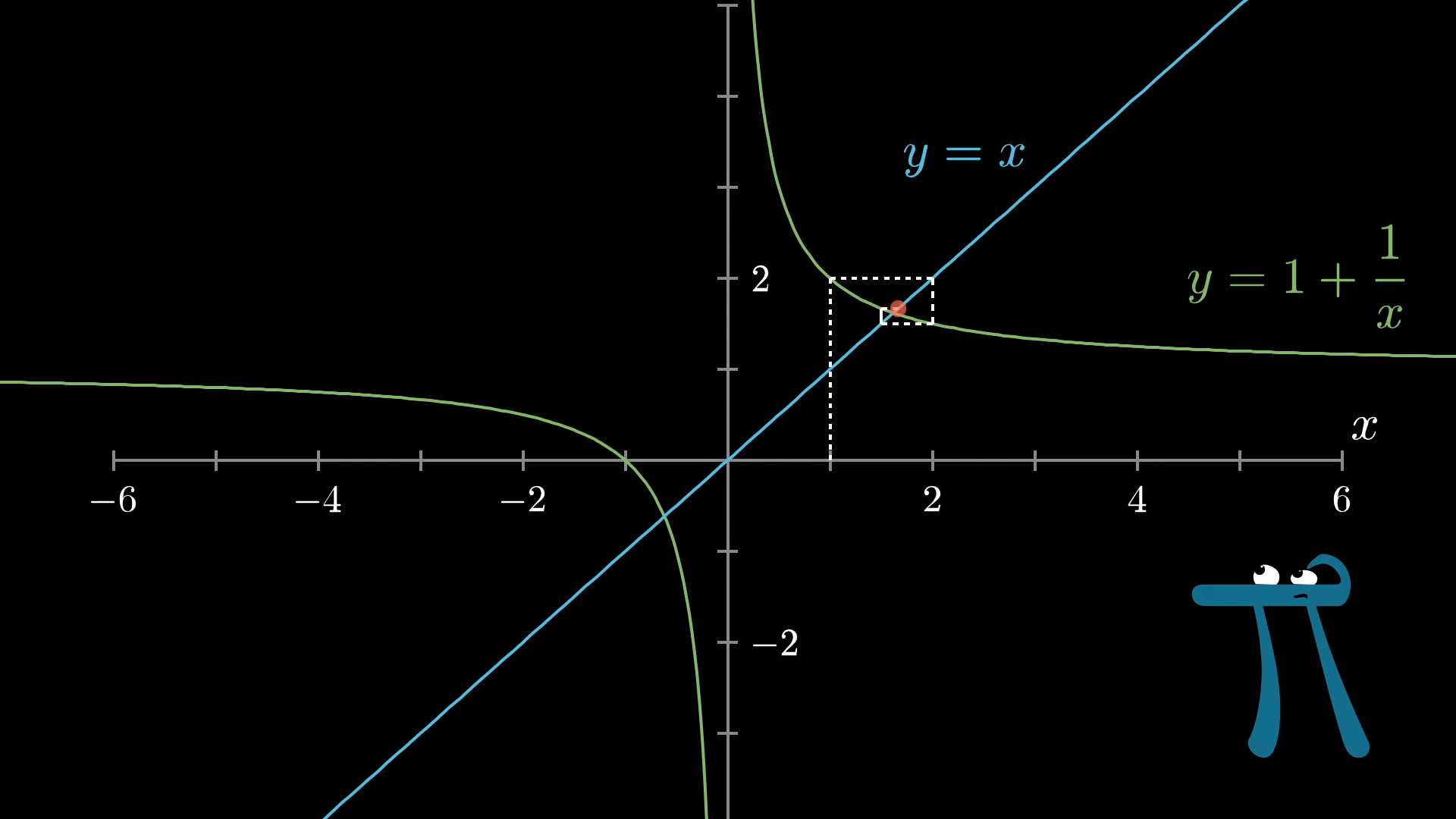
Personally, I think this is kind of an awkward way to think about repeatedly applying a function, don't you? I mean, it makes sense, but you kind of have to pause to think about it to remember which way to draw the lines. You can, if you want, think through what conditions make this spider-web process narrow in on a fixed point, vs. propagating away from it.
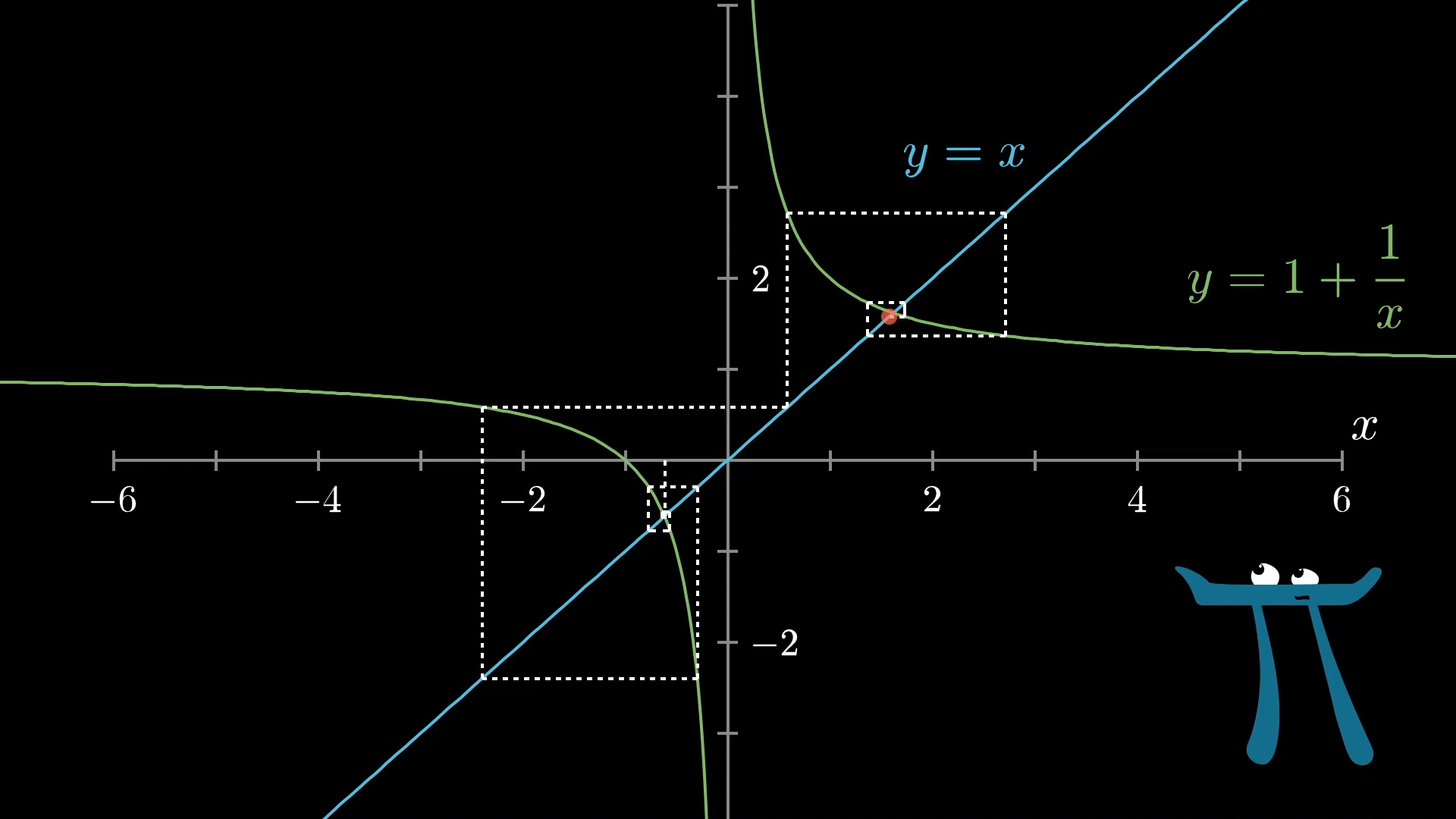
When the slope of the graph at the point where it intersects the line is relatively shallow, specifically with an absolute value less than 1, then the lines from this cobweb diagram will spiral in closer and closer to that point. But when this slope has an absolute value greater than 1, each new line drawn tends to go away from that intersection point.
But let's turn to how this function acts as a transformation.
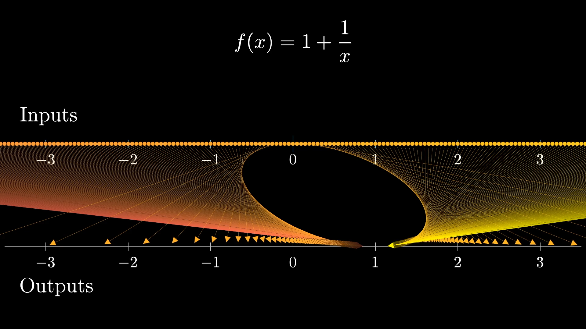
What does it look like to repeatedly apply the in this context? Well, after letting it map all input points to outputs, you consider those as the new inputs and apply that same process again and again.
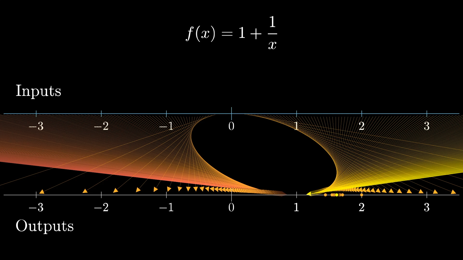
Notice how in animating this with these dots representing some sample points, it doesn't take many iterations at all for most dots to clump in around .
Now, we know that and its little brother stay fixed in place during each iteration of this process, but zoom in on the neighborhood around .
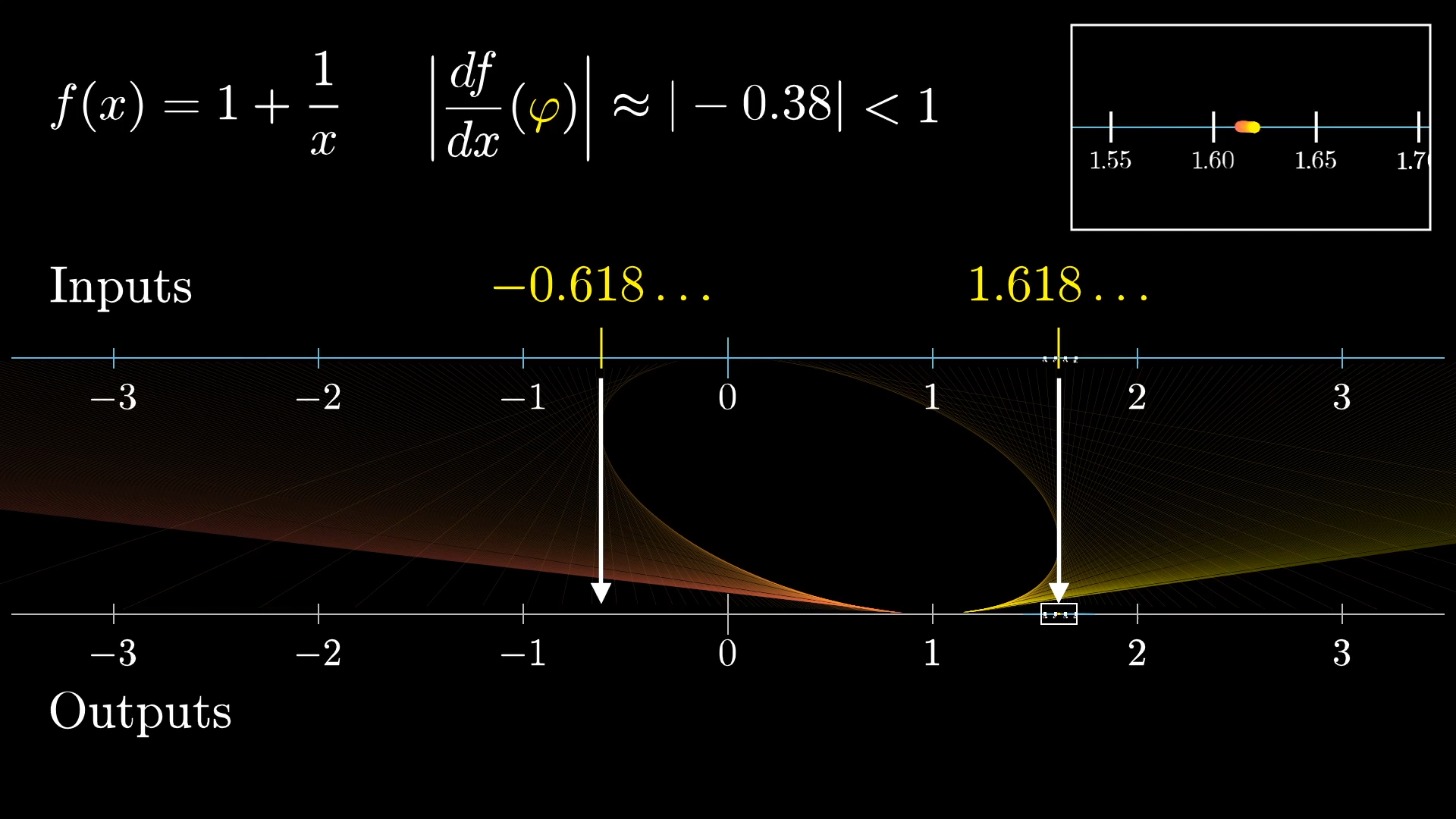
During the map, points in that region get contracted around , meaning the function has a derivative with magnitude less than 1 at the input . In fact, this derivative works out to be around at the input . So each repeated application scrunches that neighborhood smaller, like a gravitational pull towards .
So now tell me what you think happens in a neighborhood of 's little brother.
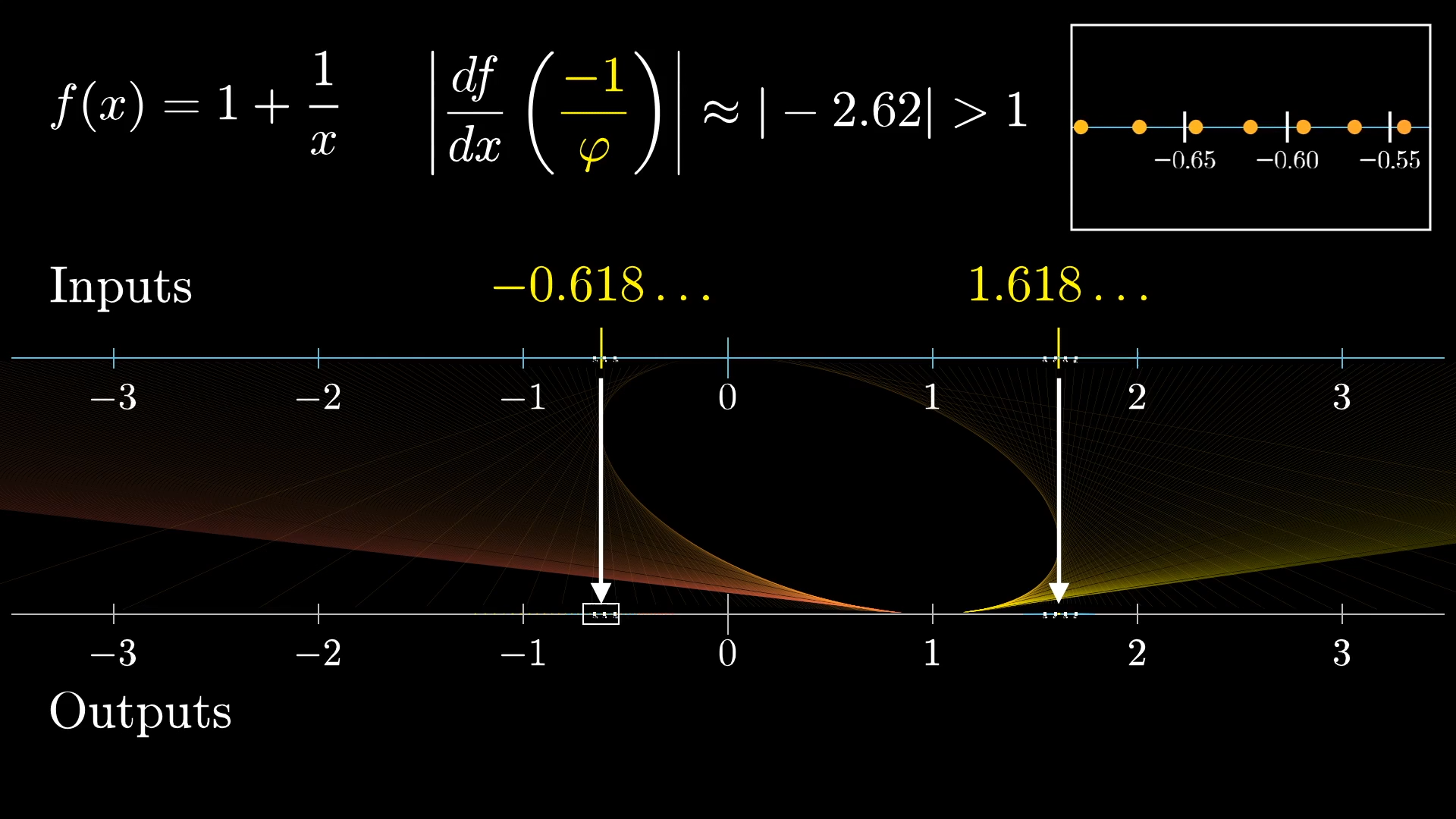
There, the derivative has a magnitude larger than , so points near this fixed point are repelled away from it, by more than a factor of each iteration. Mathematicians would call this right value a “stable” fixed point, while the left one is an “unstable fixed point”. Something is considered stable if when you perturb it a little, it tends to come back towards where it started, rather than going away.
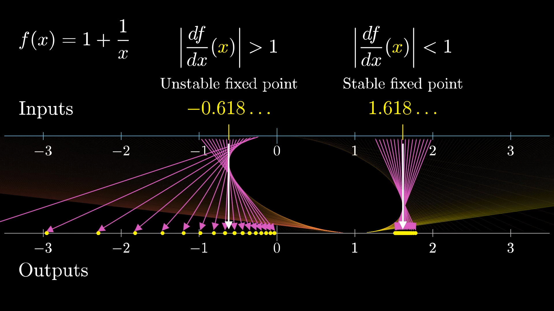
So the stability of a fixed point is determined by whether the magnitude of its derivative is bigger or smaller than , and this explains why always shows up in the numerical play, and 's little brother does not. As to whether or not you want to consider 's little brother a valid value of our infinite fraction? Well, that's really up to you. Everything we just showed suggests that if you think of this expression as representing a limiting process, only phi makes sense. But maybe you think of it not as a limit, but as a static, purely algebraic object.
Either way, math is cool!

My point here not that understanding derivatives as measuring changes in density like this is somehow better than the graphical view on the whole. In fact, picturing an entire function this way, as opposed to a small window, can be clunky and impractical as compared to graphs. My point is that it deserves more of a mention in most introductory calculus courses, and can help make a student's understanding of the derivative a little more flexible.
But as I mentioned, the real reason I'd recommend you carry this perspective with you as you learn new topics is not so much for how it will strengthen your understanding of single-variable calculus, but for what comes after. There are many topics typically taught in a college math department, which don't exactly have a reputation of being incredibly accessible.
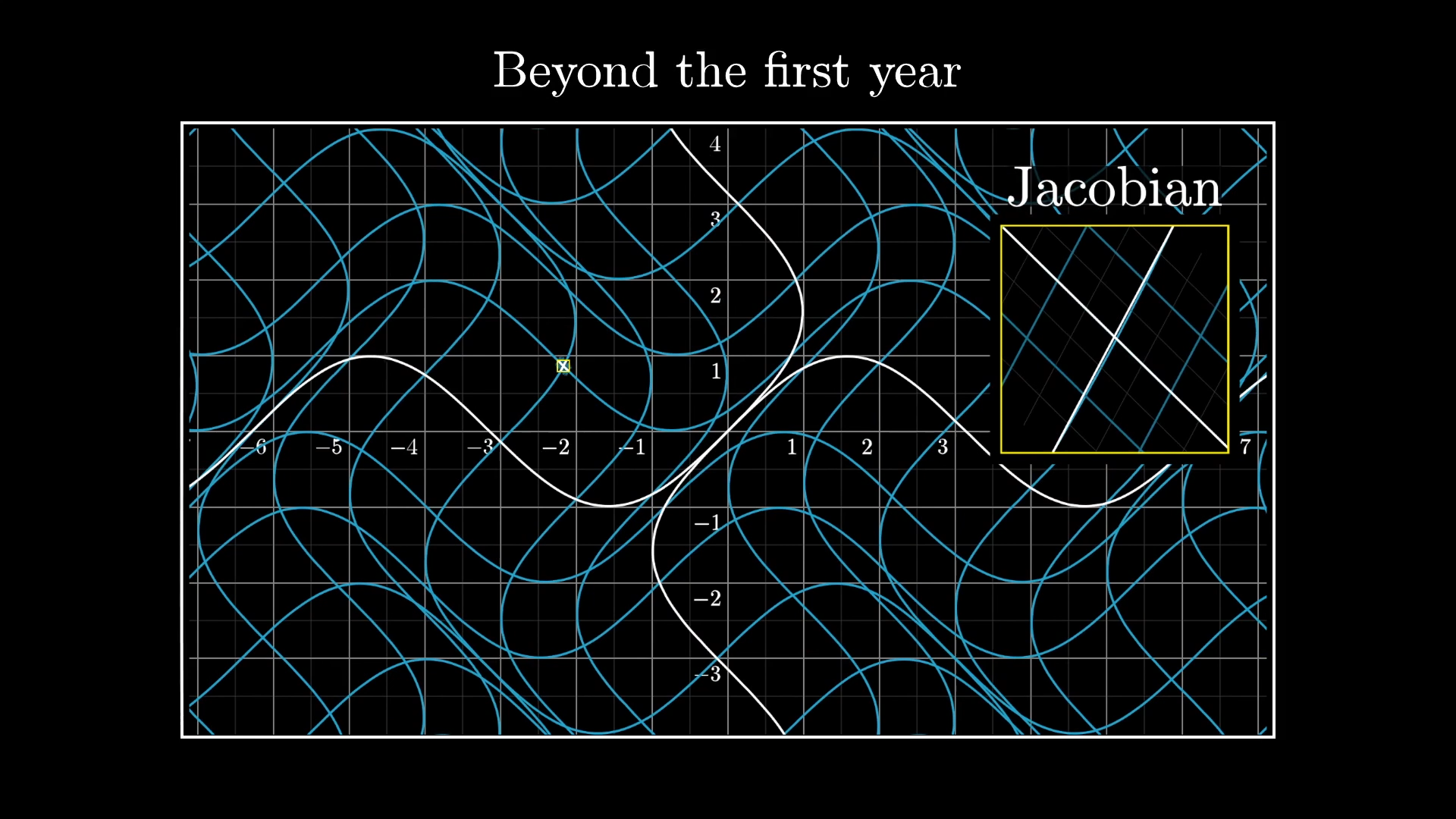
Understanding the transformation view of derivatives provides a great pathway into topics such as multivariable calculus, complex analysis and differential geometry.
Thanks
Special thanks to those below for supporting the original video behind this post, and to current patrons for funding ongoing projects. If you find these lessons valuable, consider joining.