Attention in transformers, step-by-step | Deep Learning Chapter 6
In the last chapter, you and I started to step through the internal workings of a transformer, the key piece of technology inside large language models. Transformers first hit the scene in a (now-famous) paper called Attention is All You Need, and in this chapter you and I will dig into what this attention mechanism is, by visualizing how it processes data.
Attention
Many people find the attention mechanism confusing, so before we dive into all the computational details and matrix multiplications, it's worth thinking about a couple of examples for the kind of behavior that we want it to enable.
Motivating Examples
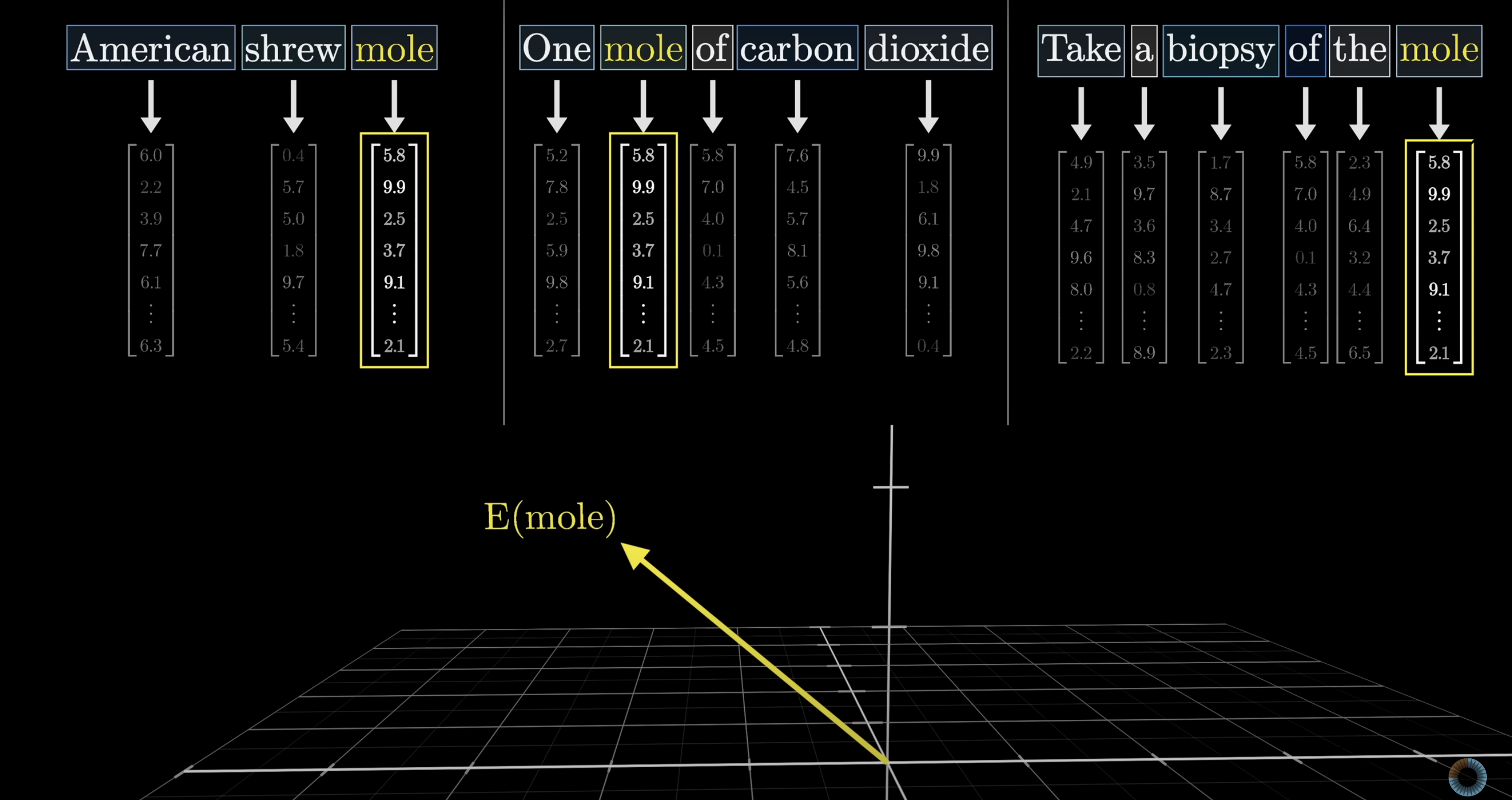
Consider these three phrases:
- American shrew mole.
- One mole of carbon dioxide.
- Take a biopsy of the mole.
You and I both know that the word mole in each of these sentences has a different meaning that's based on the context.
However, after the first step of a transformer - the embedding step that associates each token with a vector - the vector that's associated with the word mole would be the same in all of these cases, as this initial token embedding is effectively a lookup table with no reference to the context.
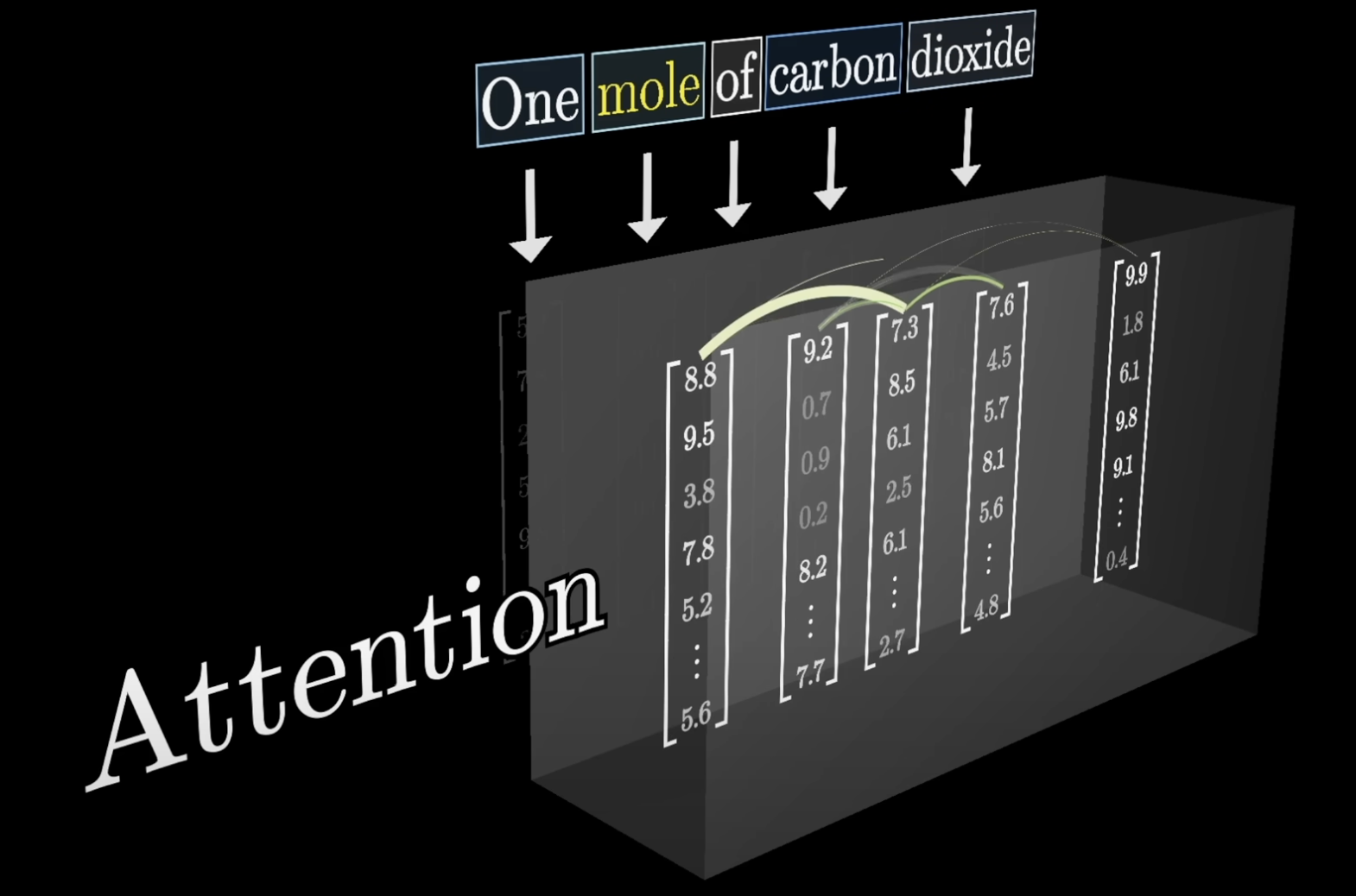
It's only in the next step of the transformer, the attention block, when the surrounding embeddings have the chance to pass information into the mole embedding and update its values.
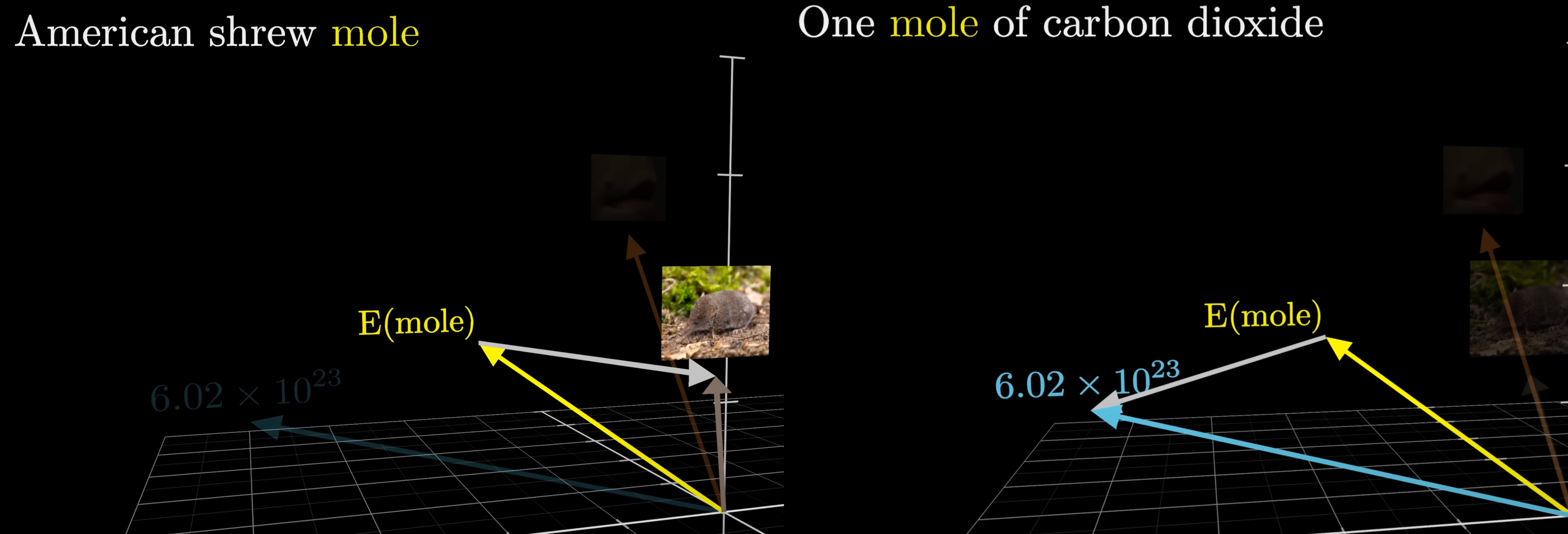
You might imagine that a well-trained model could associate multiple distinct directions in this embedding space with the multiple distinct meanings of the word mole. It is the job of an attention block to calculate what it needs to add to the generic embedding, as a function of its context, to move it to one of those specific directions.
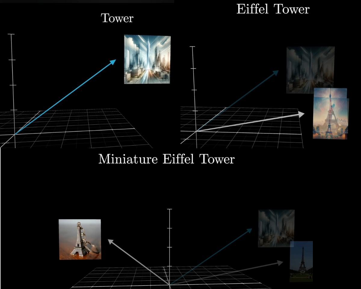
To take another example, consider the embedding of the word tower. This is presumably some very generic, non-specific direction in the space, associated with lots of other large, tall nouns.
If this word was immediately preceded by Eiffel, you could imagine wanting the mechanism to update this vector so that it points in a direction that more specifically encodes the Eiffel Tower, maybe correlated with vectors associated with Paris and France and things made of iron.
If it was also preceded by the word miniature, then the vector should be updated even further so that it no longer correlates with large, tall things.
This transfer of information from the embedding of one token to that of another can occur over potentially large distances and can involve information that’s much richer than just a single word.
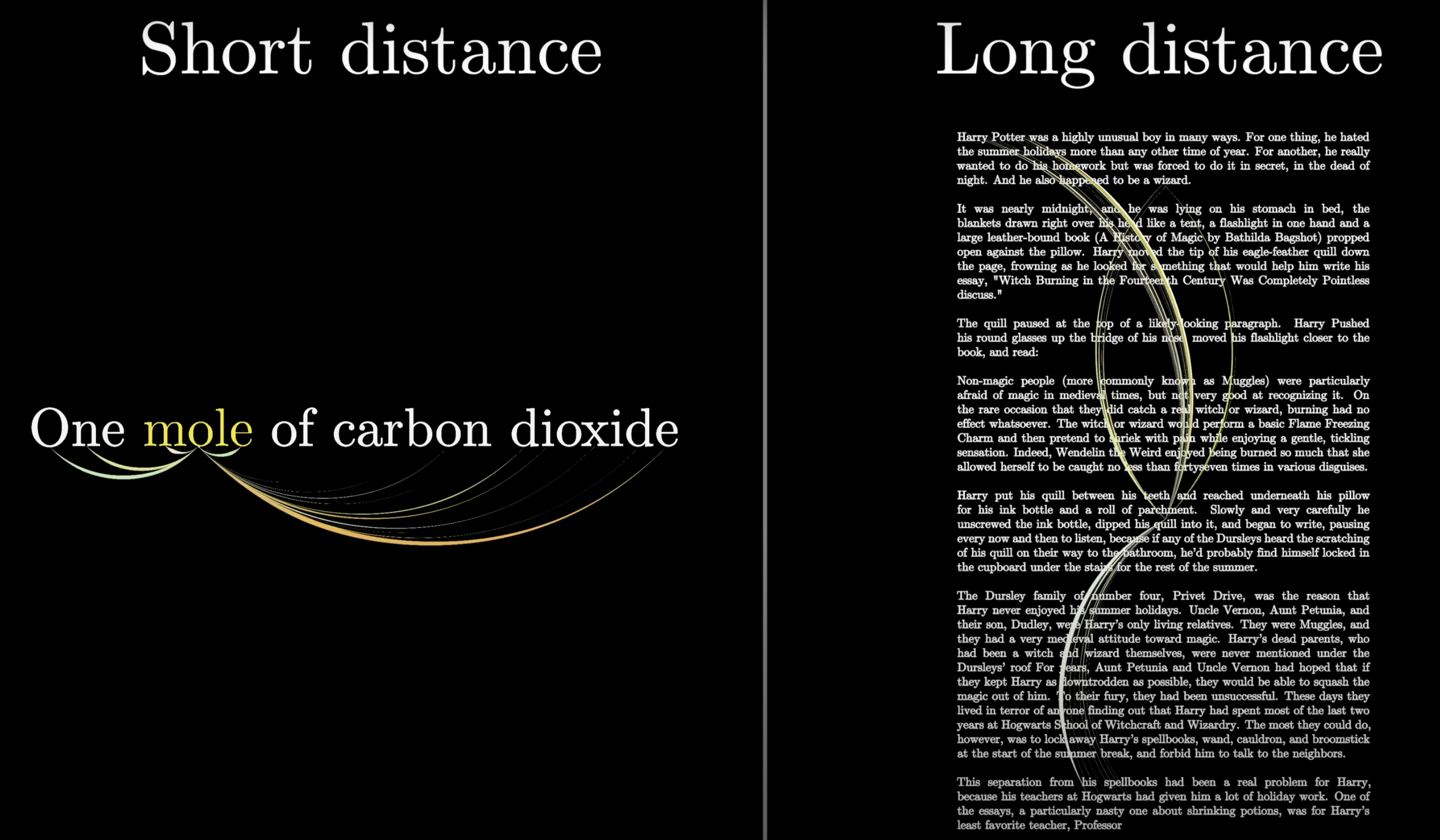
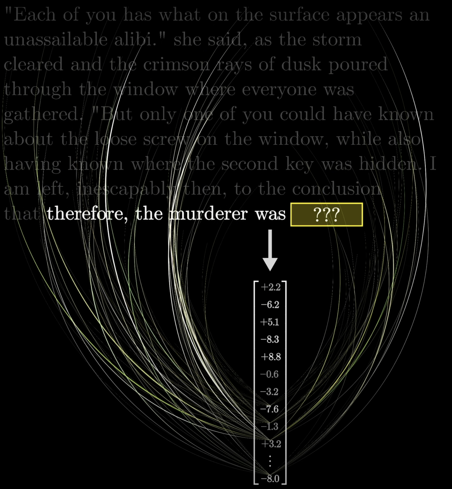
To appreciate this point, consider how in the final step of the transformer that we saw last chapter, only the last vector in the sequence is used to make the final prediction for what comes next.
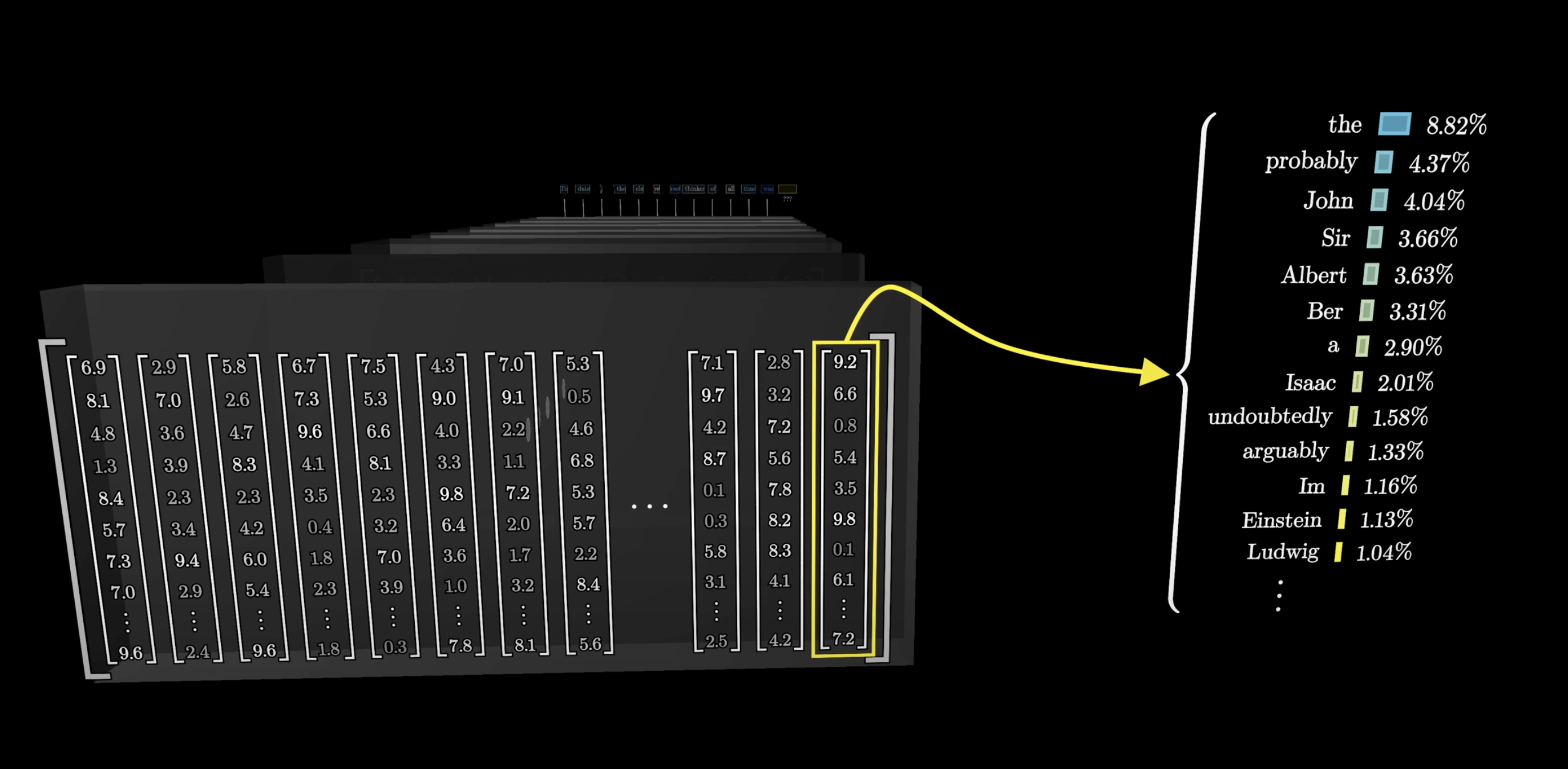
For example, imagine that the text we input was most of an entire mystery novel, all the way up to a point near the end, which reads:
Therefore the murderer was...
If the model is going to accurately predict the next word, that final vector in the sequence which began its life simply embedding the word was will have to have been updated by all of the attention blocks to represent much more than the individual word.
It will have to have somehow encoded all of the information from the full context window that's relevant to predicting the next word.
The Attention Pattern
We’ll begin by describing a single head of attention, and later we will see how the attention block consists of many different heads running in parallel.
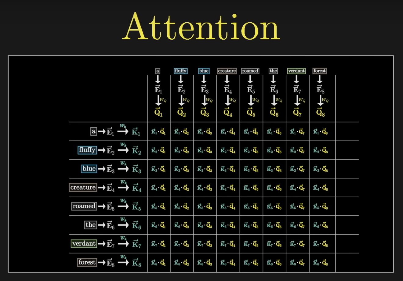
It helps to have a simple example to reference as we do this. Imagine that our input includes the phrase:
A fluffy blue creature roamed the verdant forest.
Suppose that the only type of update that we care about, for now, is having the adjectives in the phrase adjust the initial embeddings of their corresponding nouns.

Again, the initial embedding for each word is some high-dimensional vector that contains no reference to the context.
Actually, that's only partly true, as these embeddings also encode the position of the word. There's a lot more for us to say about the specific way that the positions are encoded, but for now, all we need to know is that the entries of this vector are enough to tell you both what the word is as well as where it exists in the context. Let's go ahead and denote these embeddings with the letter .
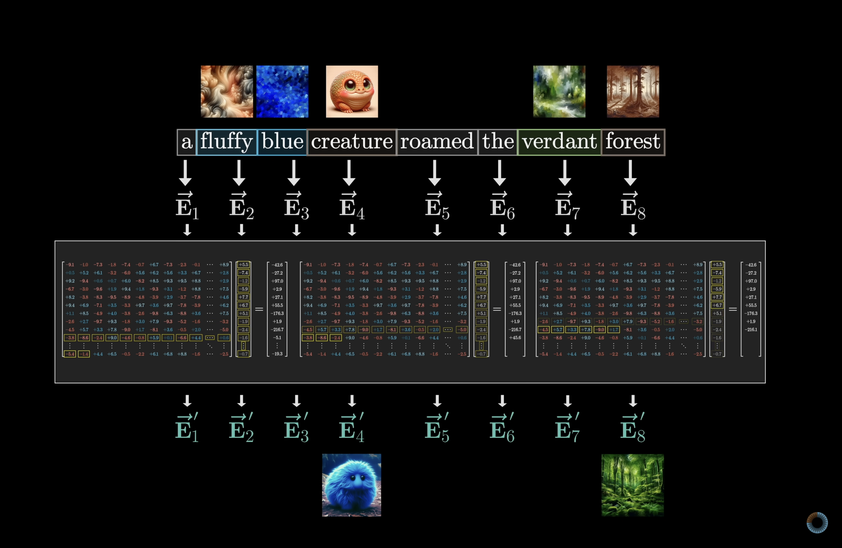
Our goal is to have a series of computations produce a new refined set of embeddings , where, in our case, those corresponding to the nouns have ingested the meaning from their corresponding adjectives.
To be clear, this example of adjectives updating nouns is just to illustrate the type of behavior that an attention head could be doing. The true behavior of an attention head is much harder to parse-as is with much of deep learning-as it’s based on the tweaking and tuning of a huge number of parameters to minimize some cost function.
As we explore all of the different matrices filled with parameters involved in this process, having a visual example of what the attention mechanism might be doing will help us keep the concepts much more concrete.
Queries
For the first step in this attention block, we can imagine each noun in the sentence asking the question:
"Hey, are there any adjectives sitting in front of me?"
These questions, like the one asked by the noun creature, are somehow encoded as yet another vector that we call the query.
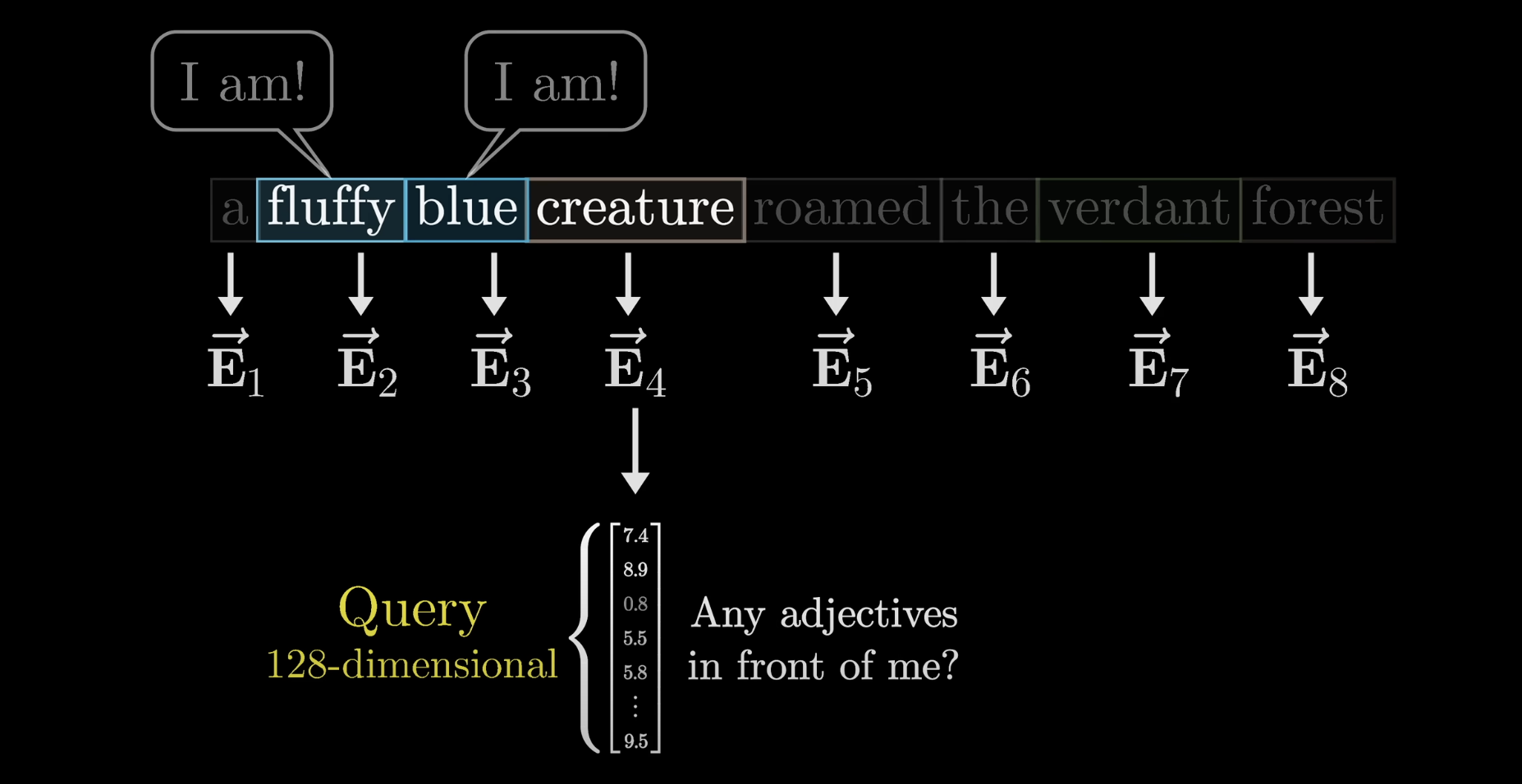
This query vector has a much smaller dimension than the embedding vector.
Computing this query looks like taking a certain matrix, which we'll label as , and multiplying it by the embedding of the word. Let's write the query vector as .
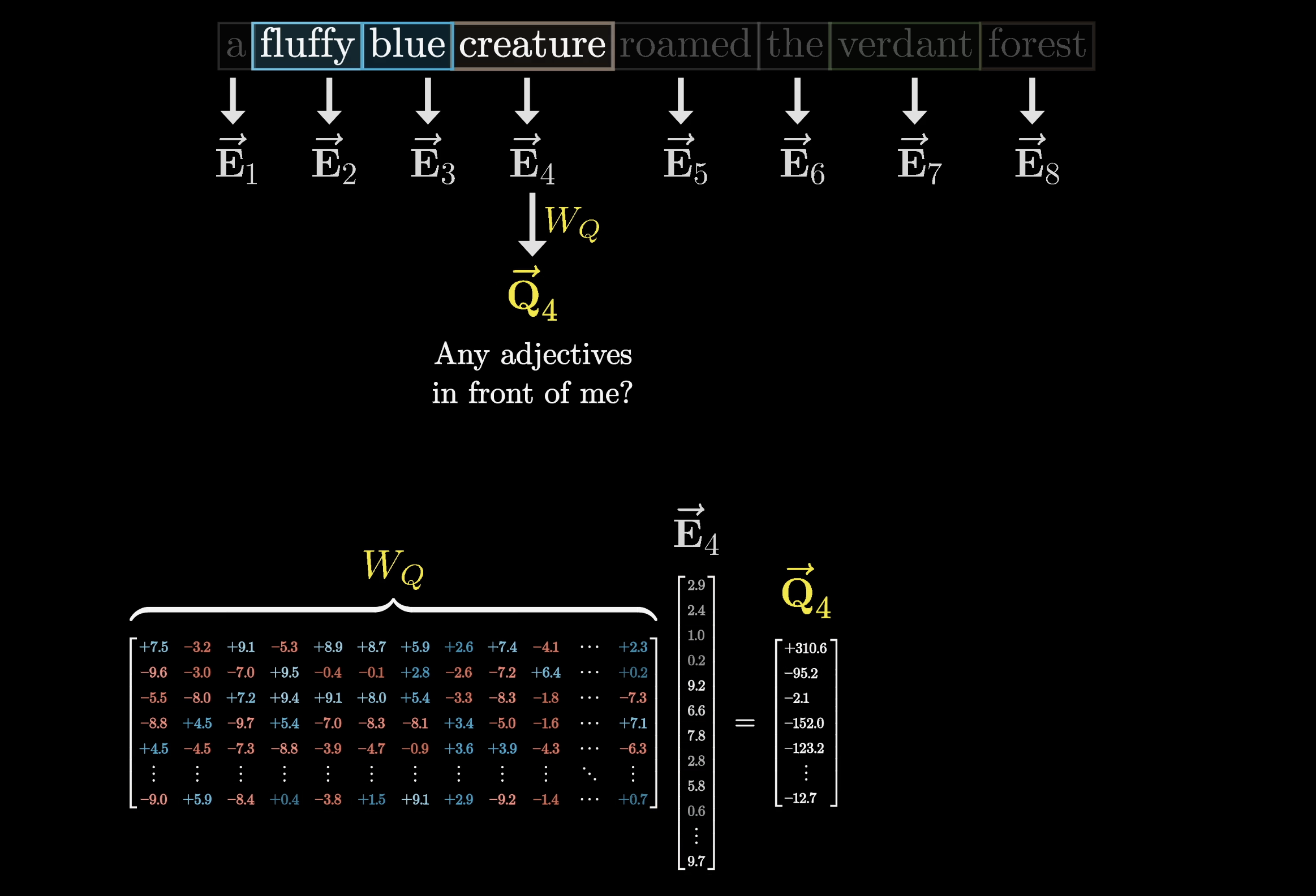
When we place a matrix next to an arrow, like in the image, it's meant to represent that multiplying the matrix by the vector at the arrow's start returns the vector at the arrow's end. In our case, we'll multiply this matrix by all of the embeddings in the context and produce one query vector for each token.
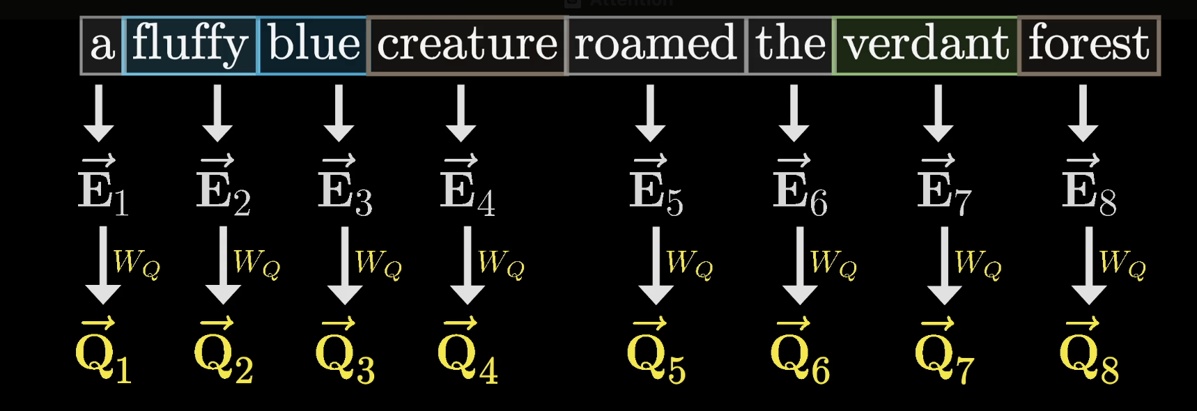
The entries of the matrix are the parameters of the model, meaning that their true behavior is learned from data. In practice, what this query matrix does in a particular attention head is challenging to parse.
Keep in mind, our nouns-and-adjectives example is made up. We’re showing one behavior that the relevant matrix operations could plausibly implement. Specifically, we’re imagining that this matrix maps the embeddings of nouns to a certain direction in this smaller query space that (somehow) encodes the notion of looking for adjectives in preceding positions.
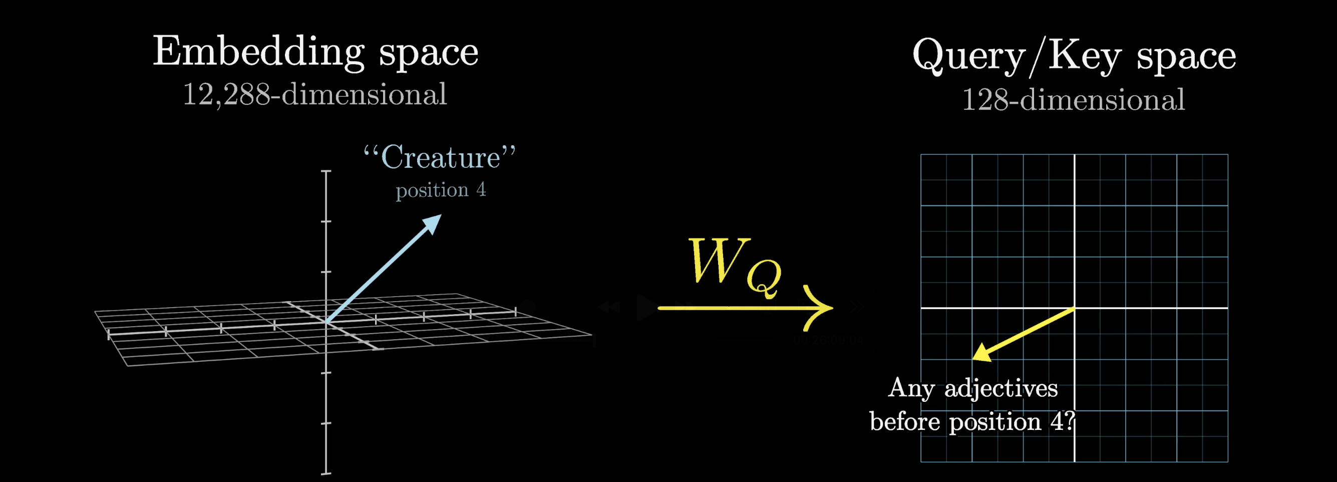
With this as our motivating example, you may very well ask: What does this matrix do to non-noun embeddings?
Who knows. Maybe it's simultaneously trying to accomplish some other goal with them. What we're focused on right now is what is happening with the nouns.
Keys
At the same time, a second matrix - the key matrix - is also multiplied by each of the embeddings. This key matrix is full of tunable parameters, just like the query matrix.
The product is a second sequence of vectors that we call the keys. Conceptually, we want to think of these keys as potential answers to the queries. We'll label the key matrix as and the keys as .
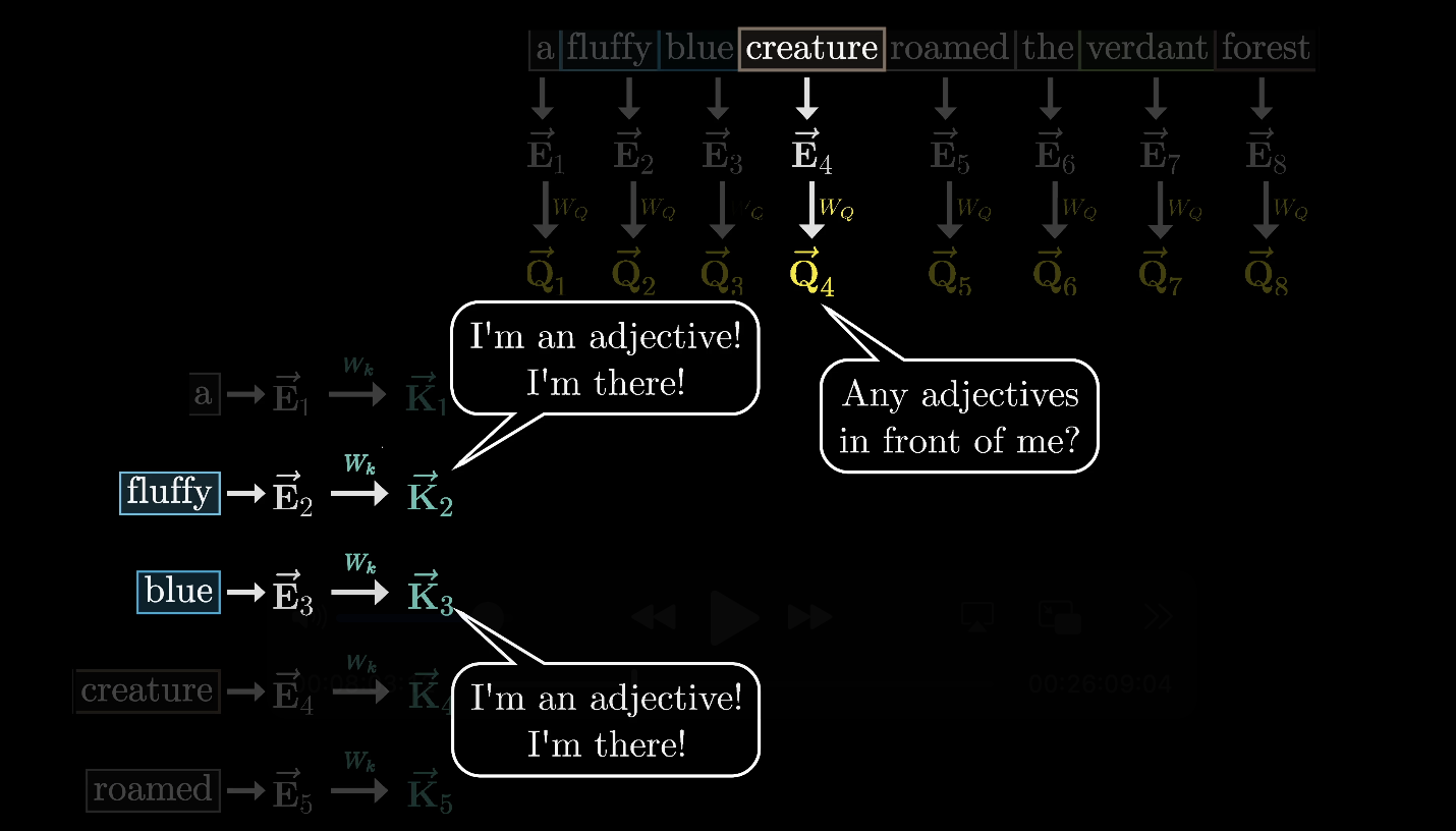
This key matrix, just like the query matrix, maps the embedding vectors to that same smaller dimensional space.
Conceptually, we want to think of the keys as matching the queries whenever they closely align with each other. In our made up example, we might imagine that the key matrix maps the adjectives like fluffy and blue to vectors that are closely aligned with the query produced by the word creature.
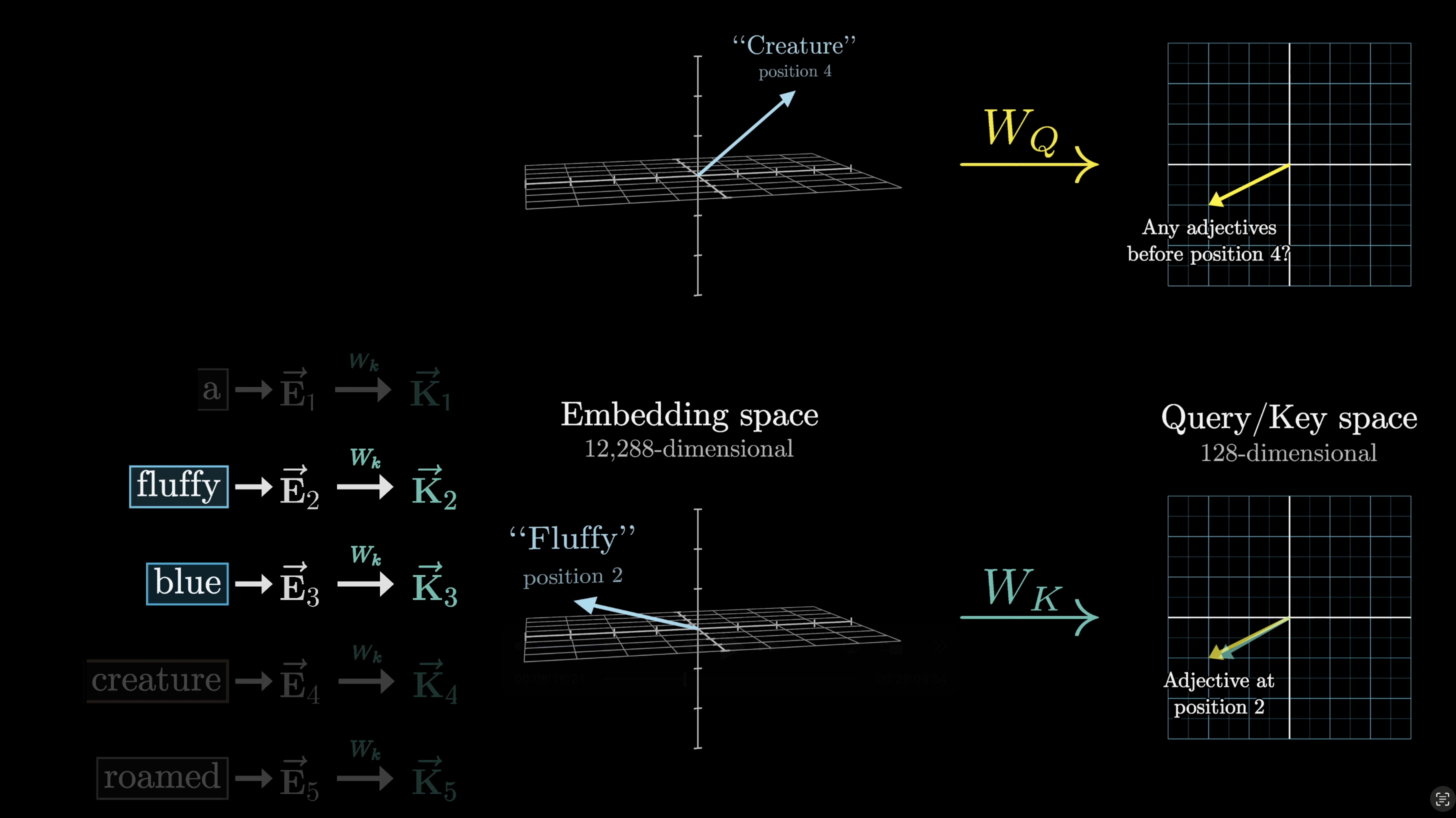
The key produced by the word fluffy is closely aligned to the query produced by the word creature.
The way we measure how closely a given pair of key and query vectors align is to take their dot product. A larger dot product corresponds to stronger alignment.
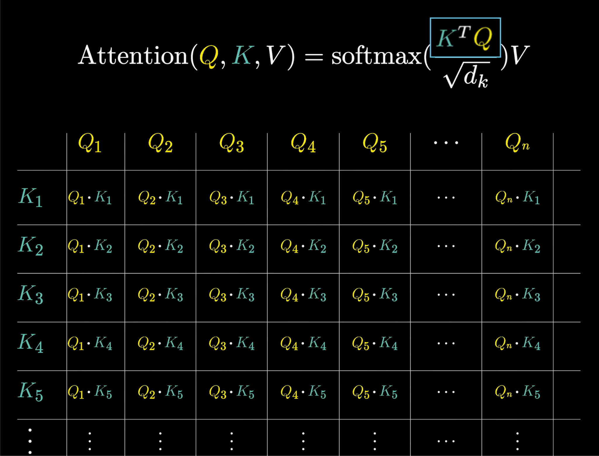
One way we could visualize this is as a grid of dots, where bigger dots correspond to larger dot products.
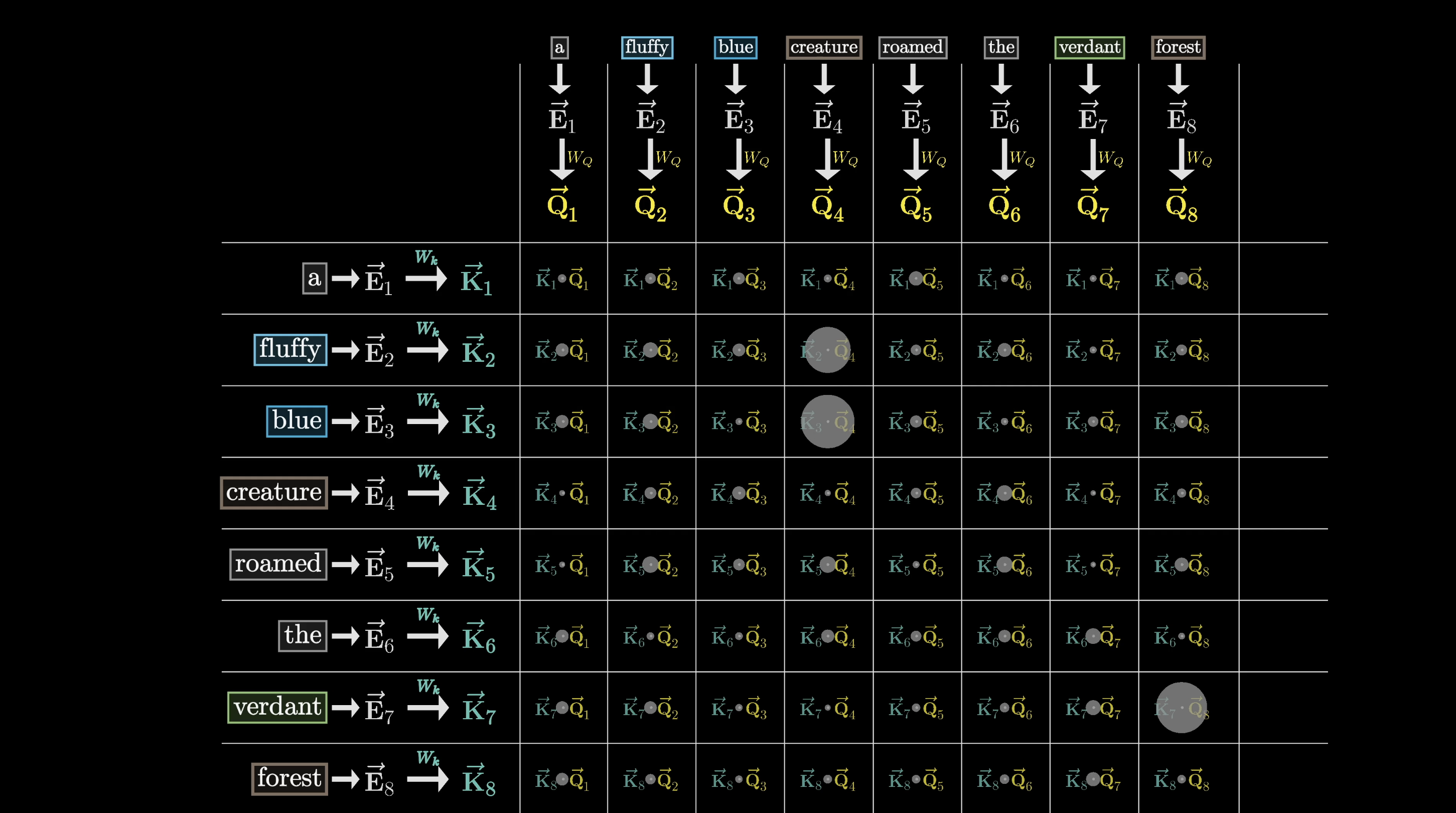
Larger dot products indicate higher alignment between the key and the query, while smaller dot products indicate weaker alignment.
In our adjective-noun example, the grid would look like the one above. The keys produced by fluffy and blue align closely with the query produced by creature, resulting in the dot products in these two spots being large, positive numbers.
In machine learning terms, this indicates that the embeddings of fluffy attend to the embeddings of creature. By contrast, the dot products between the key for some other word like the and the query for the word creature would be some small or negative value that reflects that the words are unrelated to each other.
Conceptually, the key vectors act as potential ____ to the query vectors.
After computing all the dot products of the key-query pairs, we're left with this grid, containing values ranging from to , that displays a score of how relevant each word is to updating the meaning of every other word.
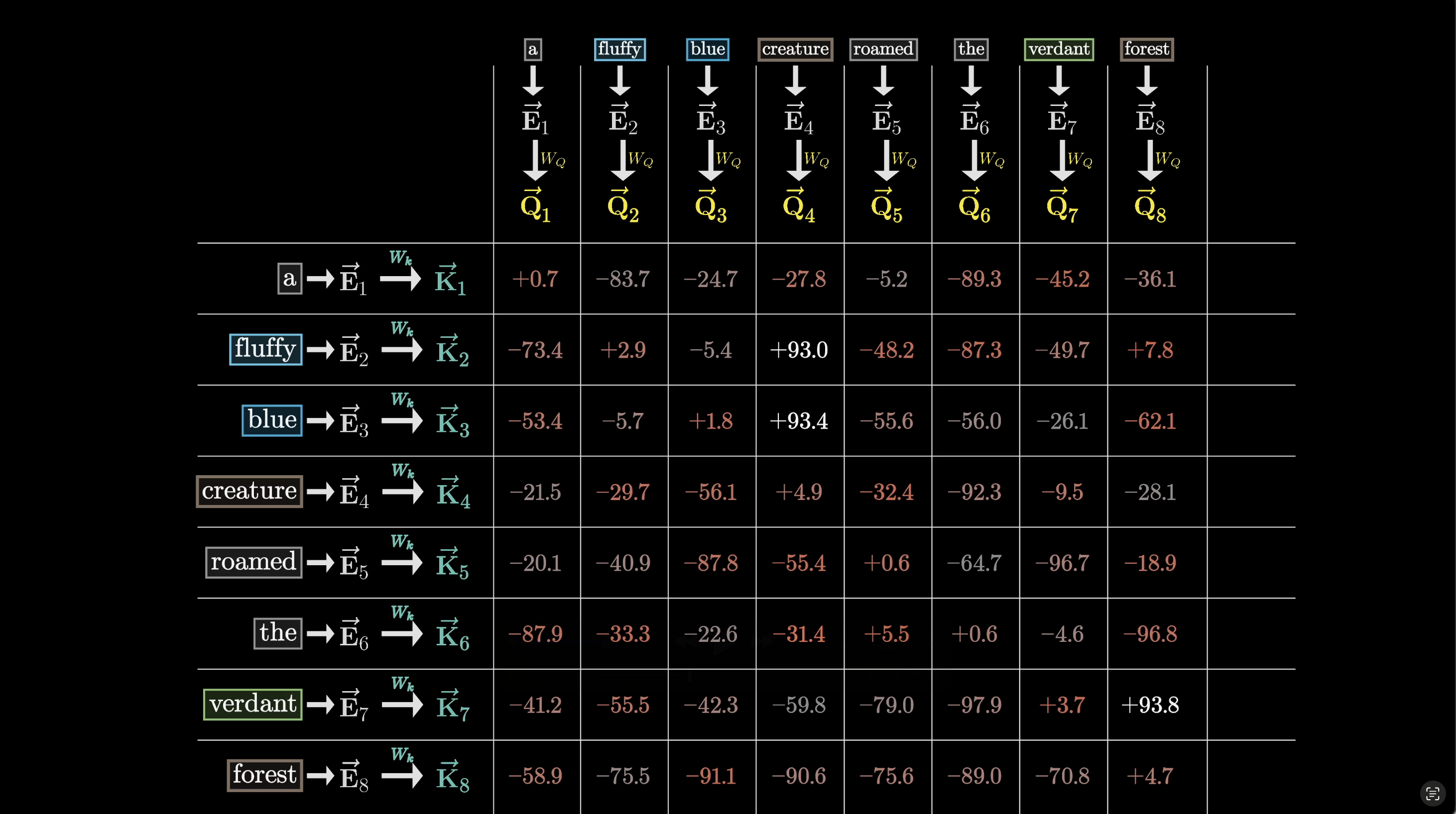
The way we're about to use these scores is by taking a certain weighted sum along each column, weighted by the relevance.
But first, instead of having values range from to , what we want is for the numbers in these columns to be between 0 and 1 and for each column to add up to 1, as if they were a probability distribution.
If you're coming from the last chapter, you're already familiar with what we need to do: compute a softmax along each one of these columns to normalize its values.
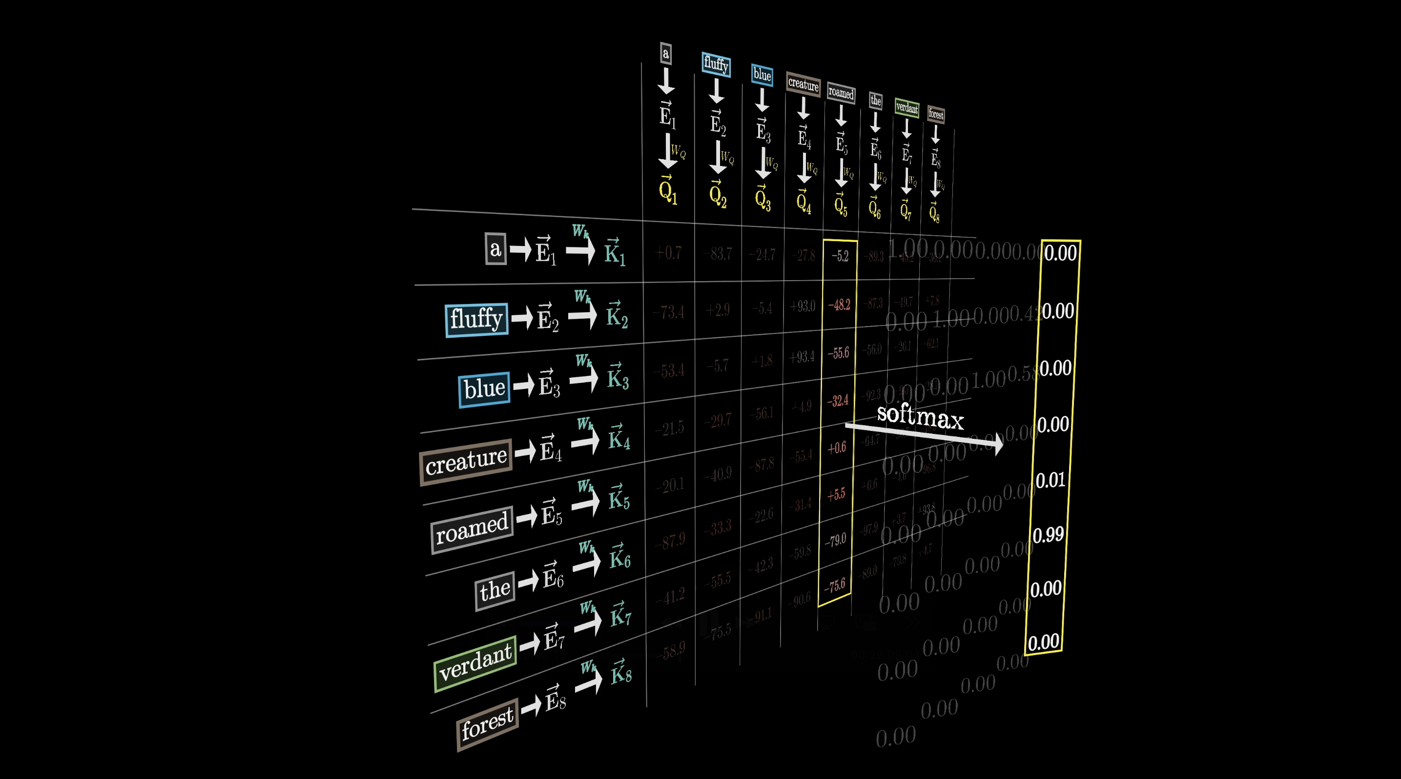
After we apply softmax to all of the columns, we'll fill in the grid with these normalized values. We call this grid the attention pattern.
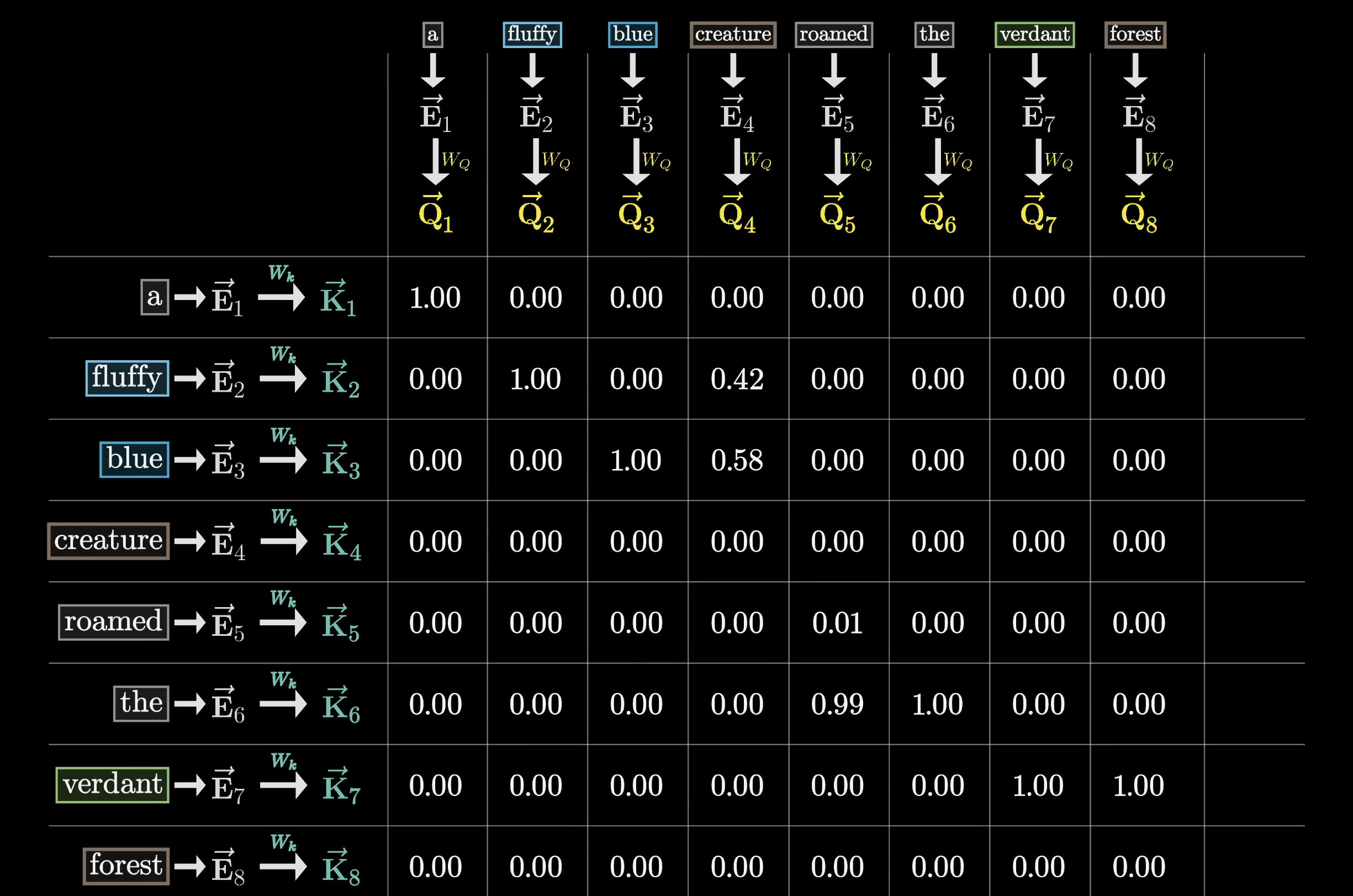
At this point, we're safe to think about each column as giving weights according to how relevant the word on the left is to the corresponding value at the top.
Based on the image, how much weight does the word blue hold relevant to the word creature?
The original transformer paper presents us with a really compact way to write this all down:
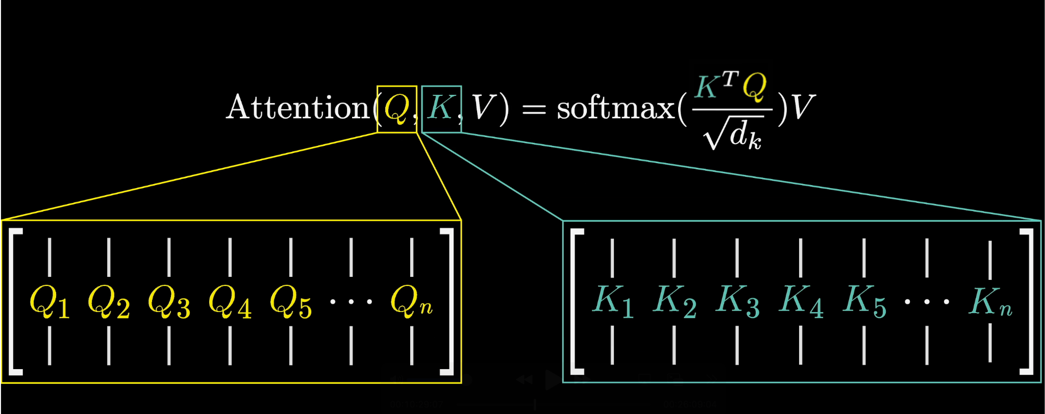
Here, the variables and represent the full arrays of query and key vectors, respectively—those smaller vectors obtained by multiplying the embeddings by the query and key matrices.
And on the right side of the equation, the numerator in the softmax function, , is a really compact way to represent the grid of all possible dot products between key-query pairs.
A small technical detail that we didn't mention is that for numerical stability, it's helpful to divide all of these values by the square root of the dimension of that key-query space, hence the denominator .
And that softmax function that's wrapped around the full expression is meant to be understood as applying softmax column by column.
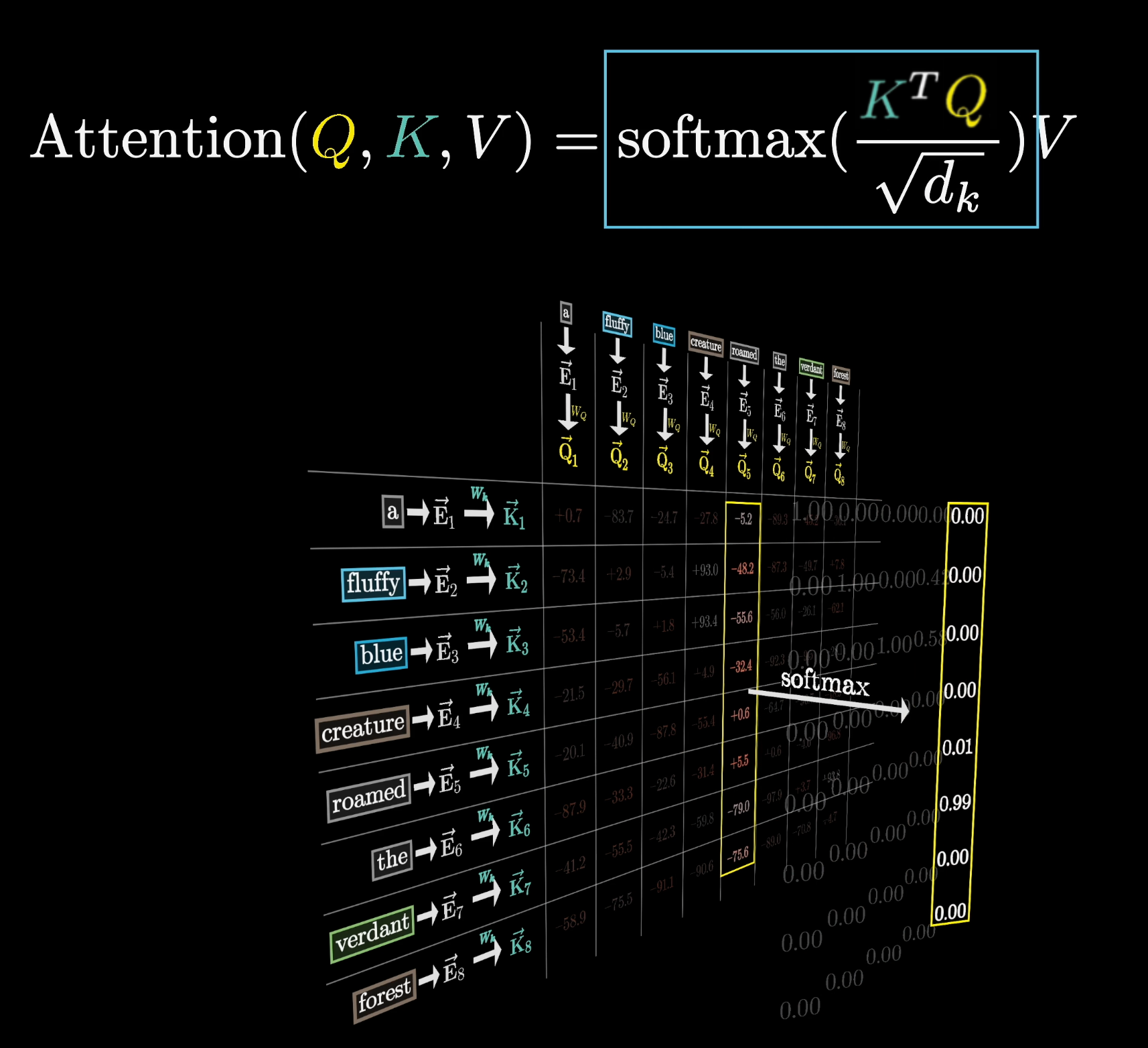
As for that term, we'll talk about it in just a second.
We've said earlier that, during the training process, the model is run on a given text example. Then the model's weights are adjusted to either reward or punish it based on the probability it assigns to the true next word.
There's actually more to it. It turns out that, to make the process more efficient, the model also simultaneously predicts every possible next token following each subsequence of tokens in the passage.
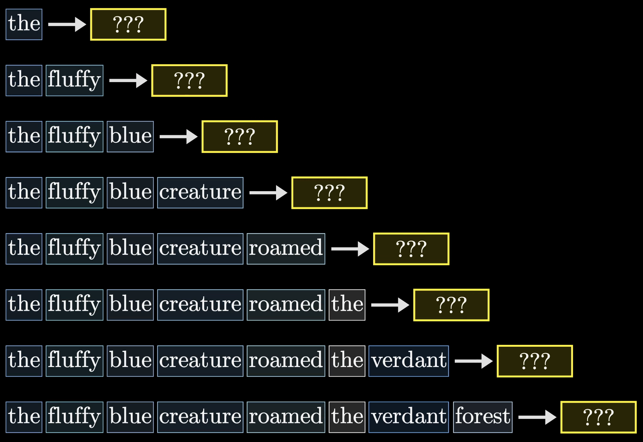
A model being trained on the phrase:
A fluffy blue creature roamed the verdant forest.
might also be predicting what words follow creature and what words follow the, and everything else along the way.
This makes the training process much more efficient, as what would otherwise be a single training example effectively acts as many.
For the purposes of our attention pattern, this also means that we would never want words that appear later in the input to influence words that appear earlier, since otherwise they could kind of give away the answer for what comes next.
In order to prevent this, what we want is for all of these spots where later tokens influence earlier ones to somehow be forced to be zero. A common way to force them to equal zero, prior to applying softmax, is to set all of those entries to be negative infinity. That way, after applying softmax, all of those spots get turned into zero, but the columns stay normalized.
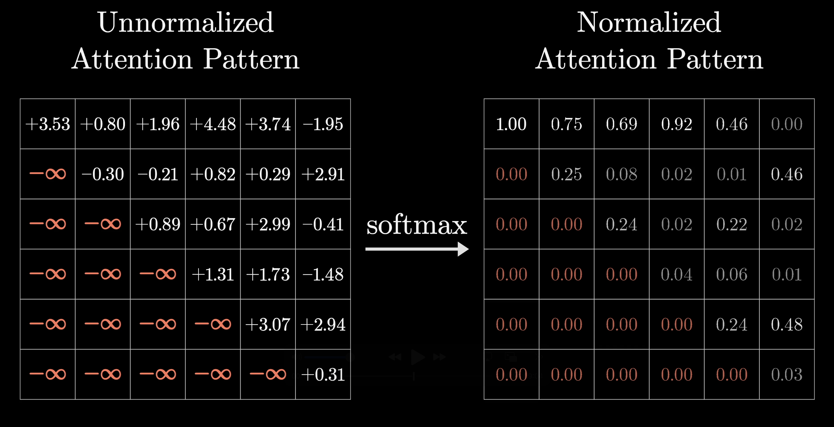
This process is called masking.
Now, there are versions of attention mechanisms where masking isn’t always applied. However, in our GPT example, masking will always be used to ensure that later tokens don’t influence earlier ones. This is especially relevant during training, though less so when the model is actually running as a chatbot.
The masking process is done to prevent ___ tokens from influencing ___ tokens.
Another fact that's worth reflecting on is how the size of this attention pattern is equal to the square of the context size.
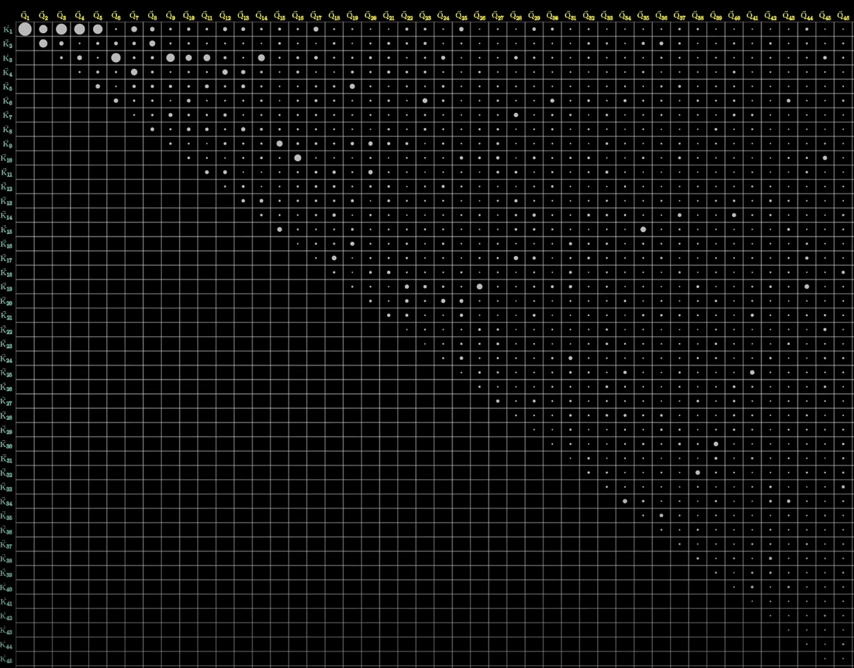
One row and one column for each token.
This is why context size could act as a significant limitation for large language models and why scaling it up is nontrivial.
Of course, motivated by a desire for larger context windows, in recent years we have seen some variations to the attention mechanism that are aimed at making context more scalable, but for now, all we're focused on are the basics.
Once you have this attention pattern describing which words are relevant to updating which other words, the next step is to actually update those embeddings.
For example, we would want the embedding of fluffy to somehow cause a change to the embedding of creature, one that moves it to a different part of this high-dimensional embedding space that more specifically encodes a fluffy creature.
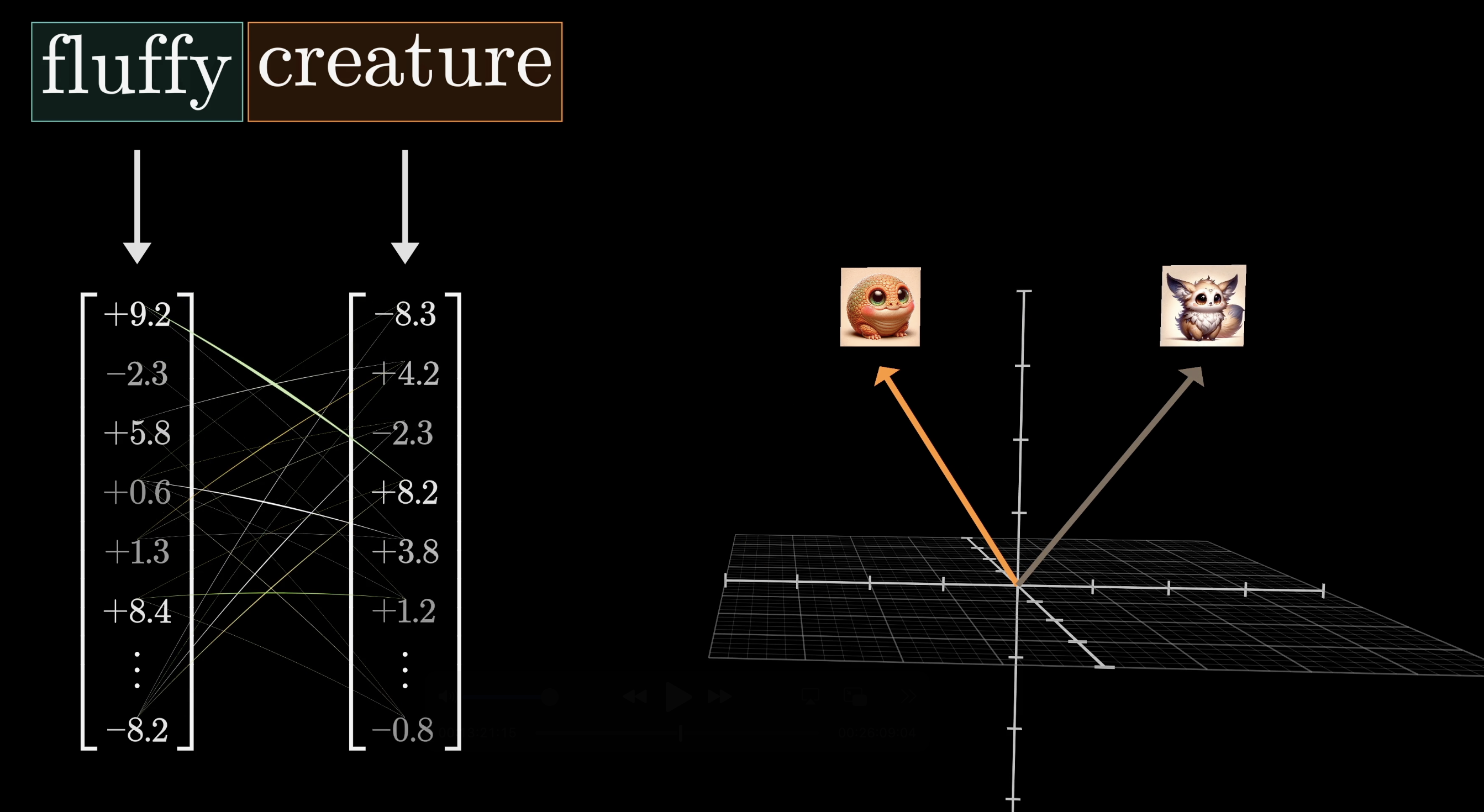
The most straightforward way would be to use a third matrix, what we call the value matrix. In true multi-headed attention, this matrix is factored into two parts, but for the moment, it’s easiest to think of as just one operation. We would multiply this value matrix by the embedding of that first word, for example fluffy. We'll denote this value matrix as .
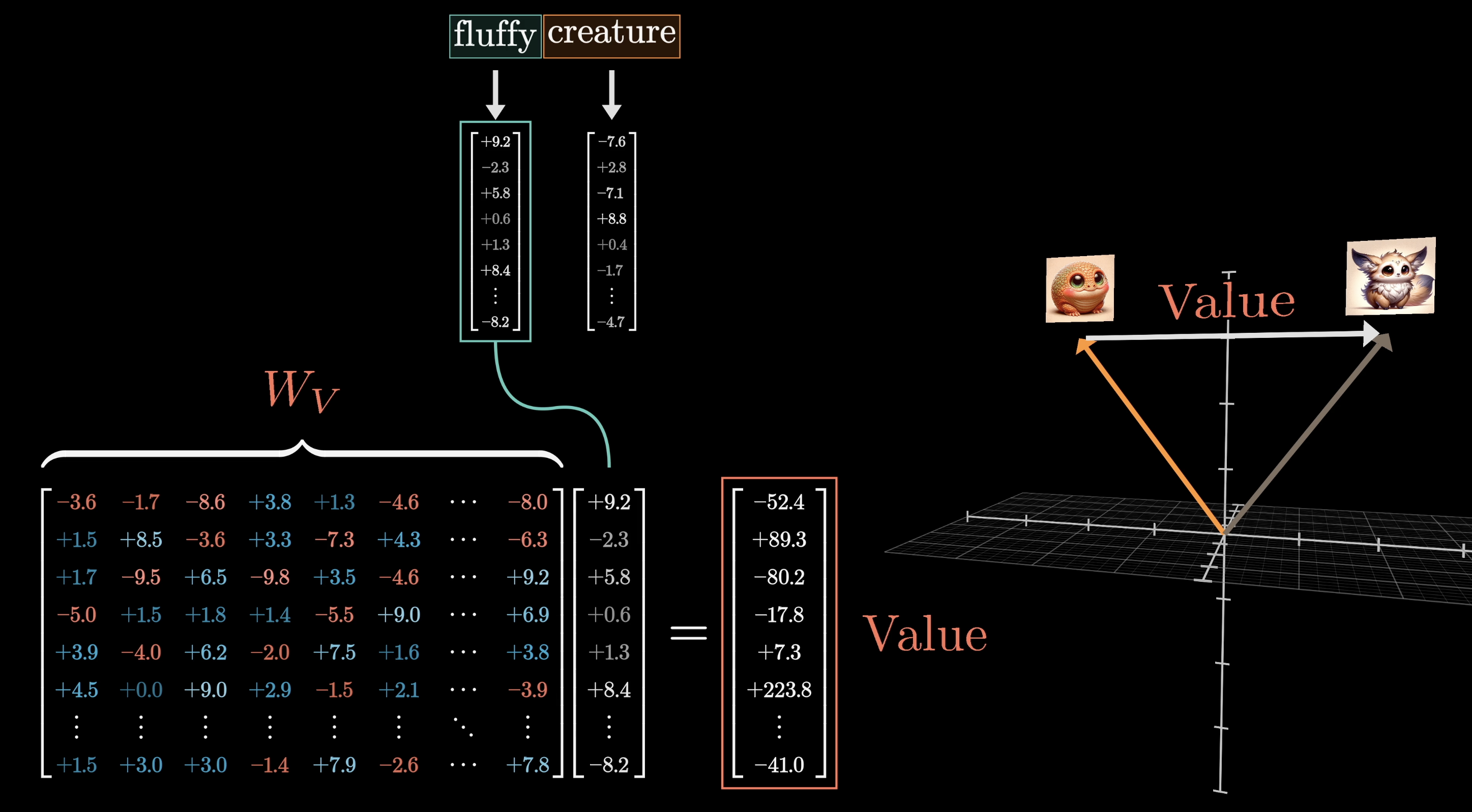
The result of this is what we would call a value vector, and this is something that we would add to the embedding of the second word. In our case, this value vector is something we would add to the embedding of creature to move it to a different part of the dimensional embedding space that encodes a fluffy creature.
This value vector lives in the same very high-dimensional space as the embeddings, and when the value matrix is multiplied by a word’s embedding, we can think of it effectively answering the question:
If this word is relevant to adjusting the meaning of another word, what specific adjustments should be made to the other word's embedding to reflect this relevance accurately?
This value matrix is multiplied by every one of those embeddings to produce a sequence of value vectors.
We might think of these value vectors as being associated with the corresponding keys. For each column in our grid, we would multiply each of the value vectors by the corresponding weight in that column.
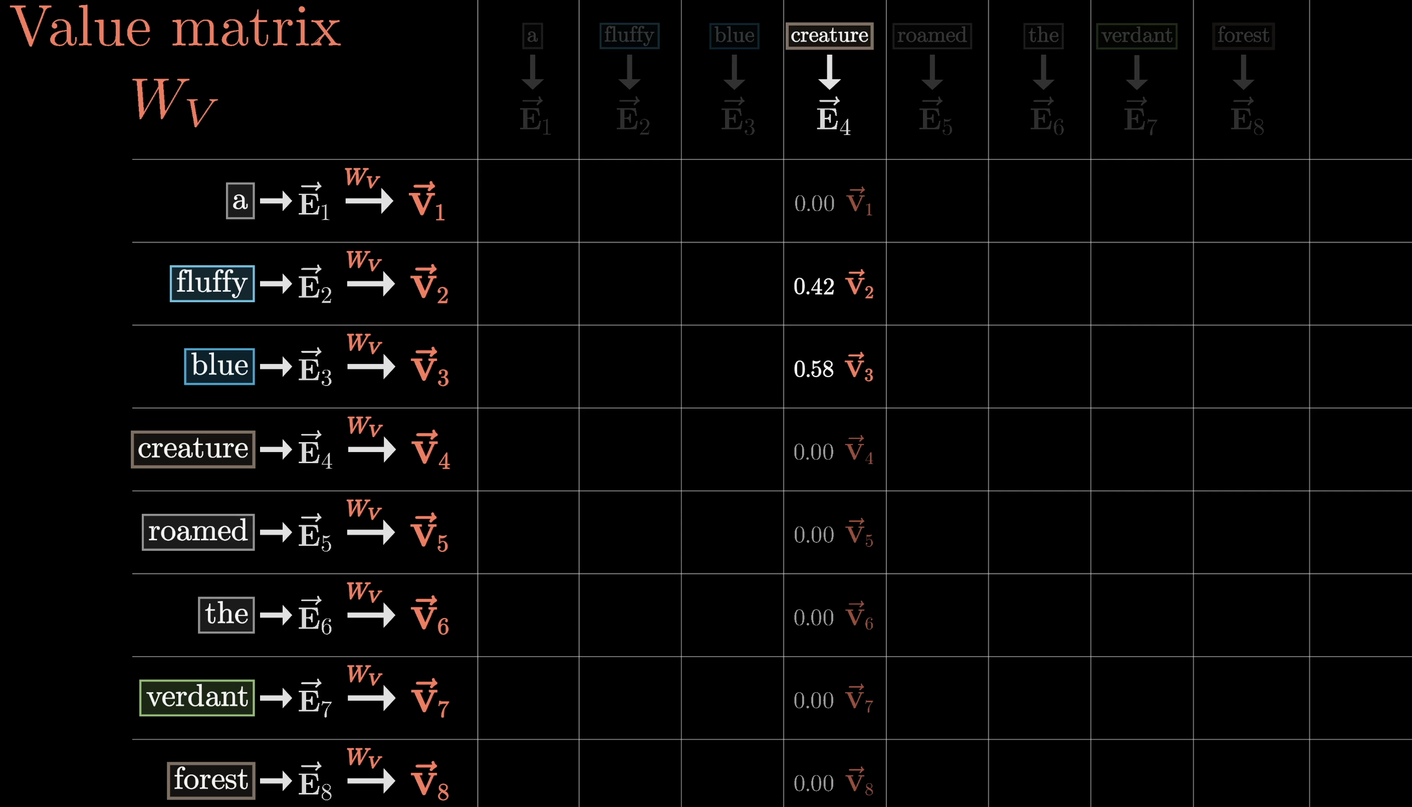
Under the embedding of Creature, we would be adding large proportions of the value vectors for fluffy and blue, while all of the other value vectors get nearly zeroed out.
Then finally, the way we actually update the embedding associated with this column, previously encoding some context-free meaning of creature, is by adding together all of these rescaled values in the column.
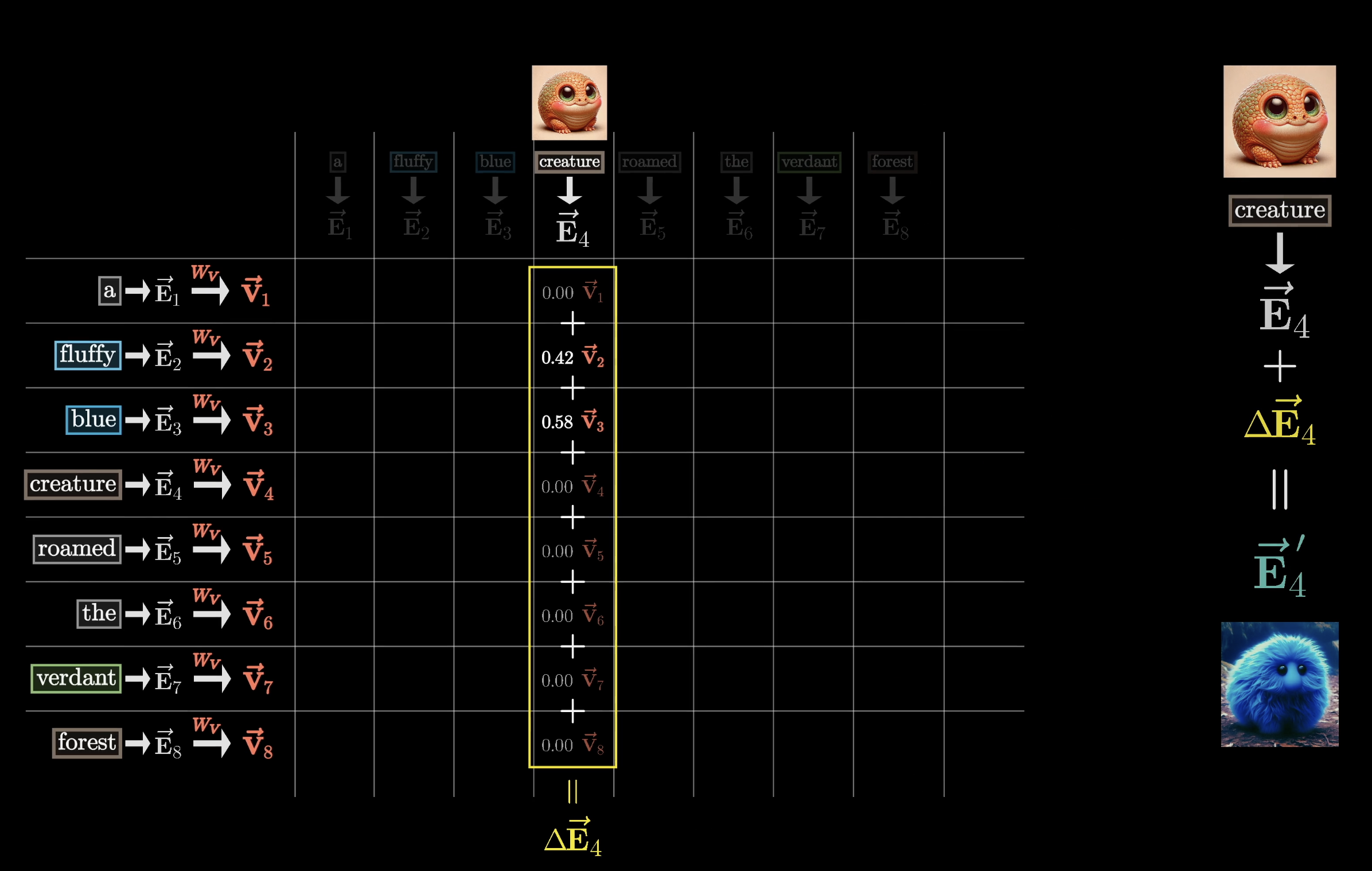
This produces the change that we want to add, which we'll label as . Then, adding this to the original embedding hopefully results in a refined vector that encodes a much more contextually rich meaning, like a fluffy blue creature in our example.
Of course, this process isn't only done with one embedding. We would apply the same weighted sum across all of the columns in this picture, producing a sequence of changes. When adding all of those changes to the corresponding embeddings, they produce a full sequence of more refined embeddings popping out of the attention block.
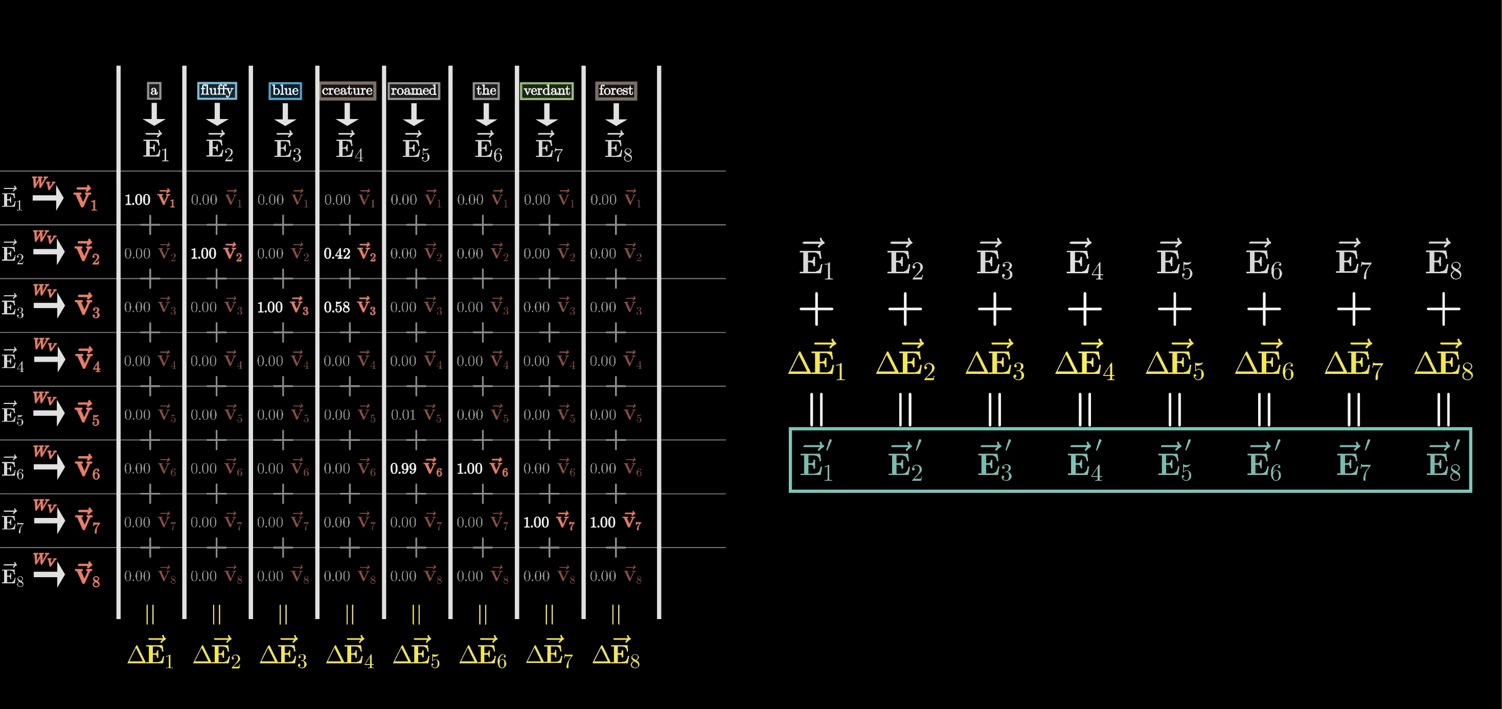
Zooming out, this whole process is what we would describe as a single head of attention.
To summarize, this single head of attention is parameterized by three distinct matrices: the key matrix, the query matrix, and the value matrix, all filled with tunable parameters.
Counting Parameters
Let's take a moment to continue what we started in the last chapter and count up the total number of model parameters using the numbers from GPT-3.
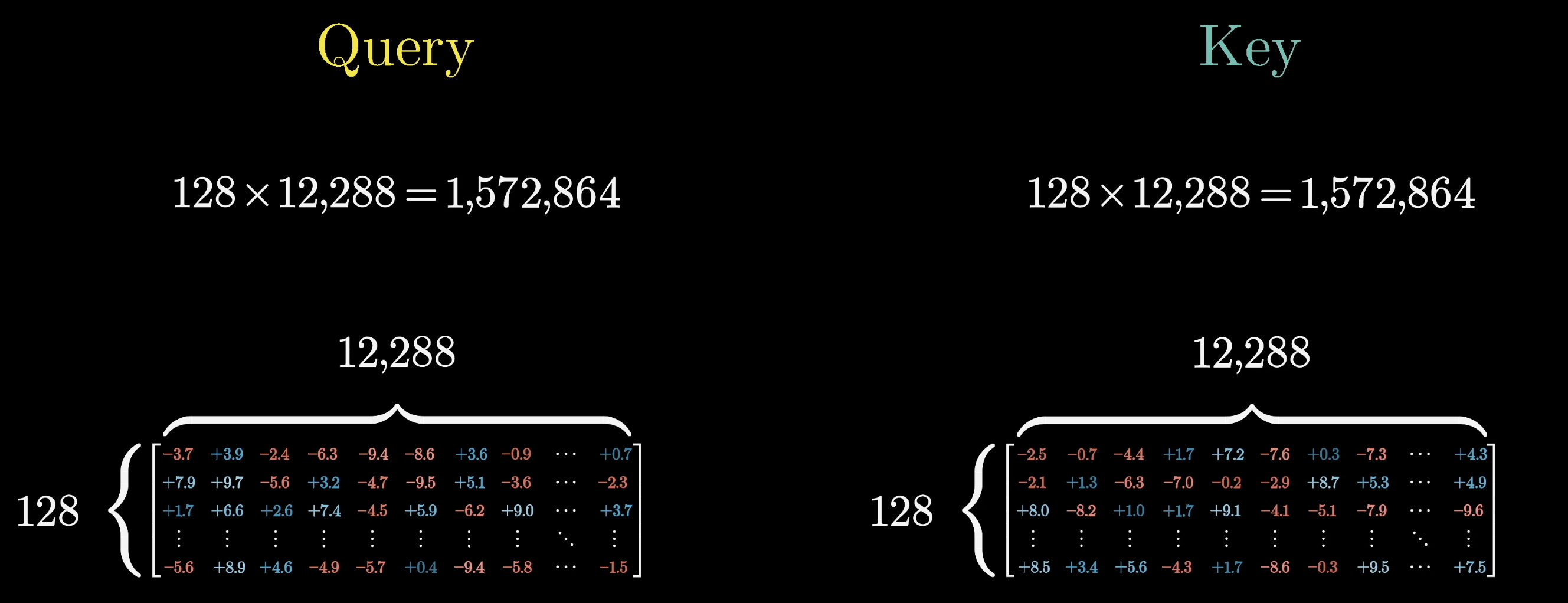
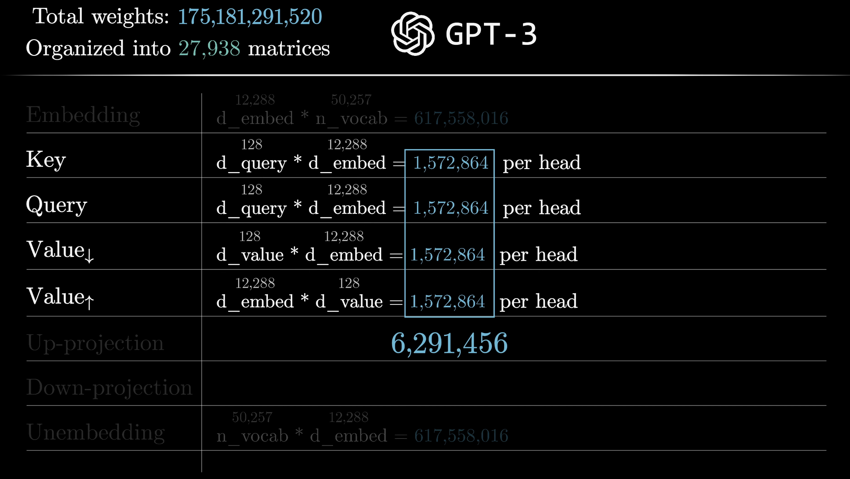
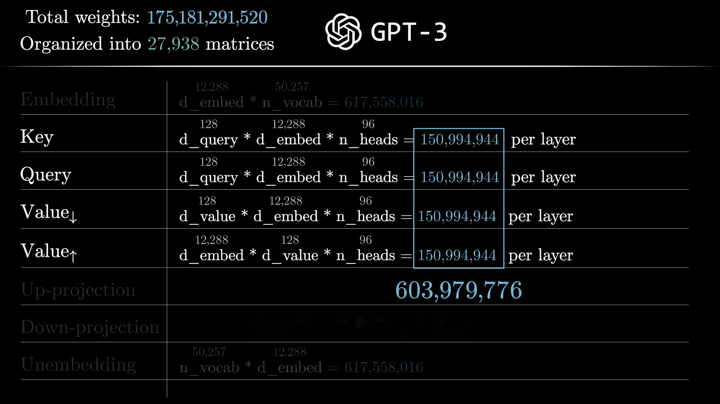
In GPT-3, the key and query matrices each have 12,288 columns, matching the embedding dimension, and 128 rows, matching the dimension of that smaller key-query space. This gives us an additional 1,572,864 parameters for each matrix.
Looking at that value matrix, the way we've described things so far would suggest that it's a square matrix that has 12,288 columns and 12,288 rows, since both its inputs and outputs live in the very large embedding space. If this were true, that would mean 150,994,944 added parameters, which is way more than the added parameters for the key and query matrices.
While we could devote that many parameters to the value map, in practice it's much more efficient to make it so the amount of parameters devoted to the value matrix is equal to that devoted to the query and key matrices.

This is especially relevant in the setting of running multiple attention heads in parallel. The way this looks is that the value map is factored as a product of two smaller matrices.
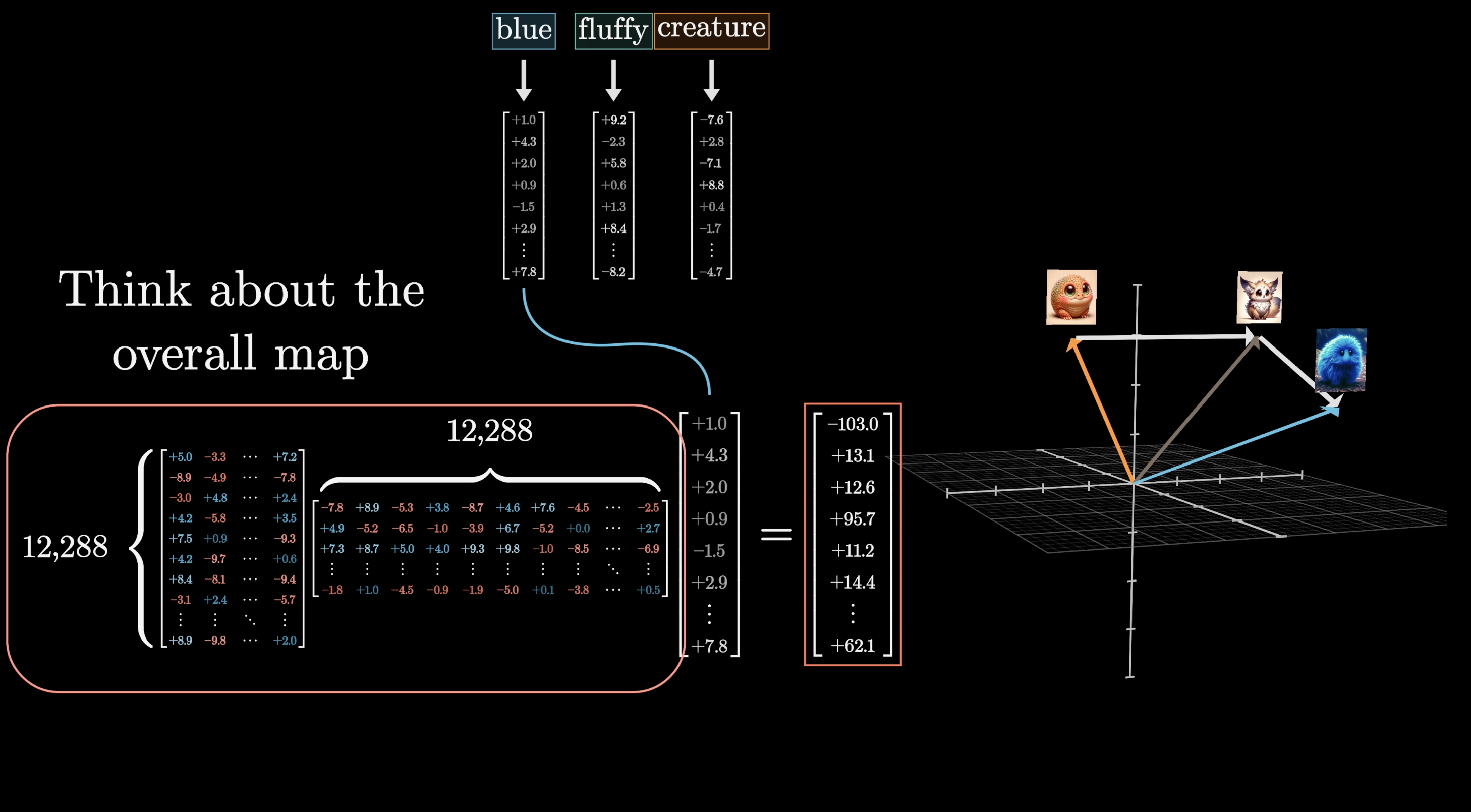
Conceptually, we should still think about the overall linear map, one with inputs and outputs, both in this larger embedding space, just broken up into two different steps.
The matrix on the right, the one with 12,288 columns, has the smaller number of rows, typically the same size as the key-query space, which in our case is 128. We can think of this as mapping the large embedding vectors down to a much smaller space. We'll call this the matrix for now, though note that it isn't the conventional name.
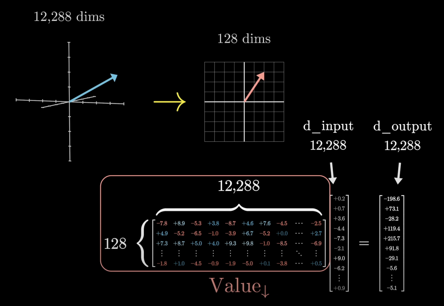
The second matrix maps from this smaller space back up to the embedding space, producing the vectors that you use to make the actual updates. We're going to refer to this matrix as the matrix, which again isn't the conventional name.
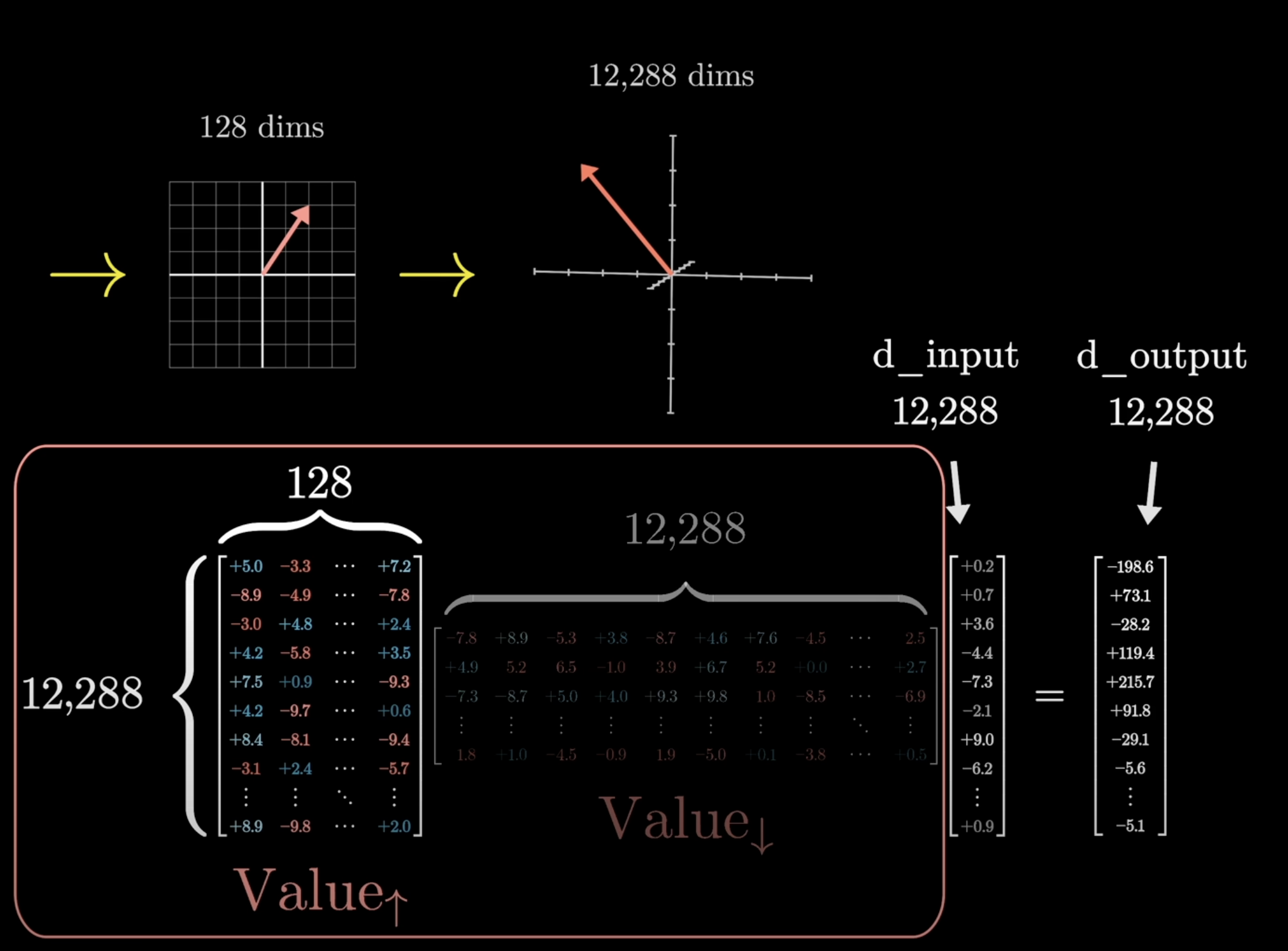
In Linear Algebra terms, what we're essentially doing is constraining the overall value map to be a low-rank transformation.
The way this is written in most papers looks a little different and tends to make things a little more conceptually confusing. We'll go over why that's the case later.
Going back to the parameter count, all four of these matrices have the same size, and adding them all up gets about 6.3 million parameters for one attention head.
If you've understood everything so far and were to stop here, you would go with an understanding of the essence of what attention really is. All that's really left for us to do is to understand the idea that this process is repeated many, many different times across many, many different attention blocks(and MLPs), all within a transformer.
In our central example we focused on adjectives updating nouns, but of course there are lots of different ways that context can influence the meaning of a word.
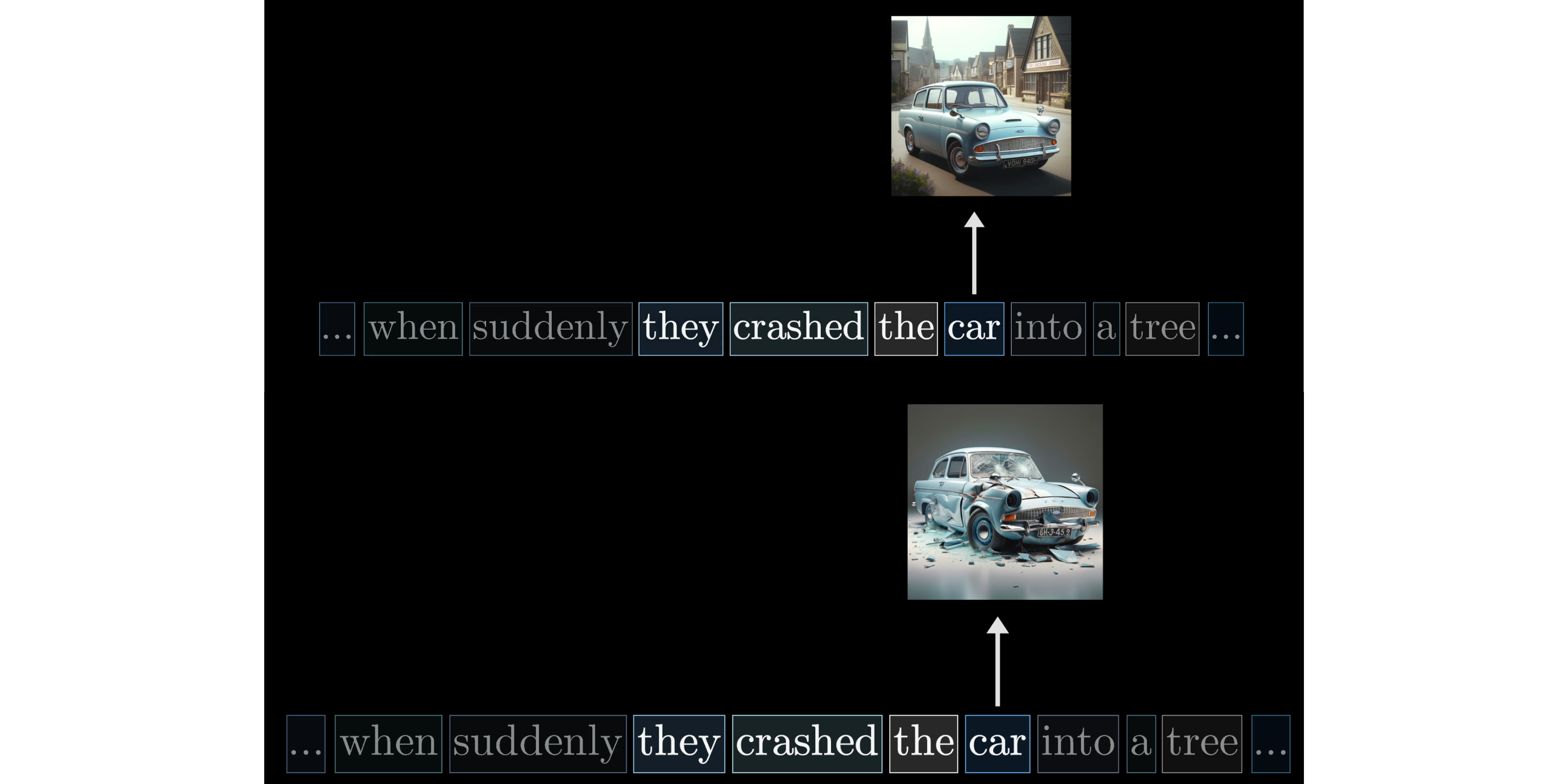
For example, if the words they crashed the preceded the word car, it has implications for the shape and structure of that car.
Or a lot of associations might be less grammatical. If the word wizard is anywhere in the same passage as Harry, it suggests that this might be referring to Harry Potter, whereas if instead the words Queen, Sussex, and William were in that passage, then perhaps the embedding of Harry should instead be updated to refer to the prince.
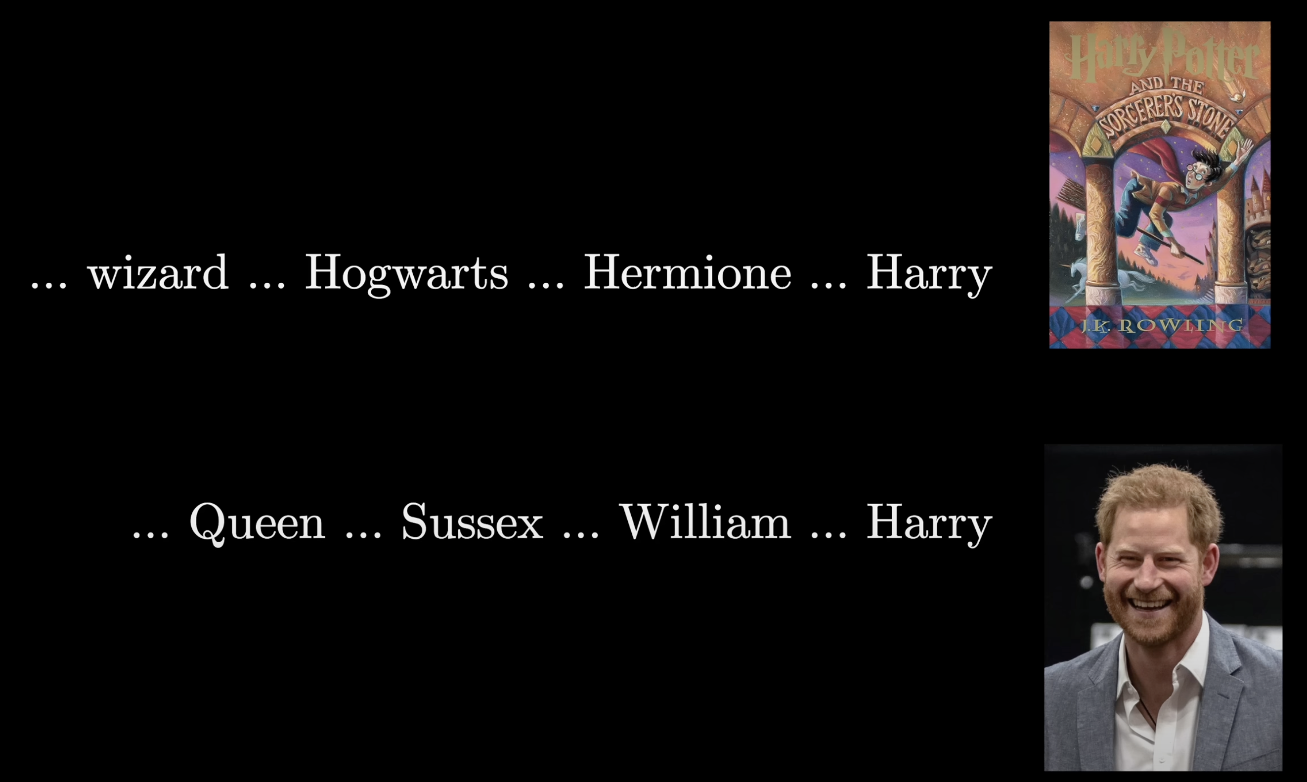
The point is, for every different type of contextual updating that we might imagine, the parameters of these key and query matrices would be different to capture the different attention patterns, and the parameters of our value map would be different based on what should be added to the embeddings.
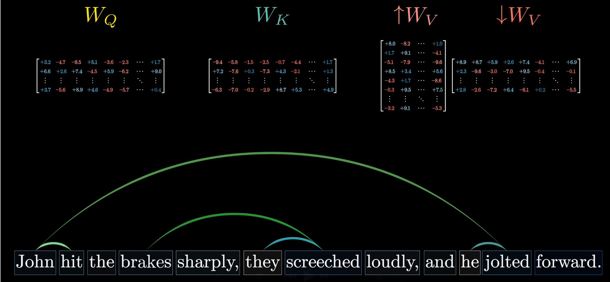
Again, in practice the true behavior of these maps is much more difficult to interpret, where the weights are set to do whatever the model needs them to do to best accomplish its goal of predicting the next token.
All the content we've covered so far is all contained in a single head of attention. A full attention block consists of what's called a multi-headed attention, where a lot of these operations are run in parallel, each with its own distinct key, query, and value maps.
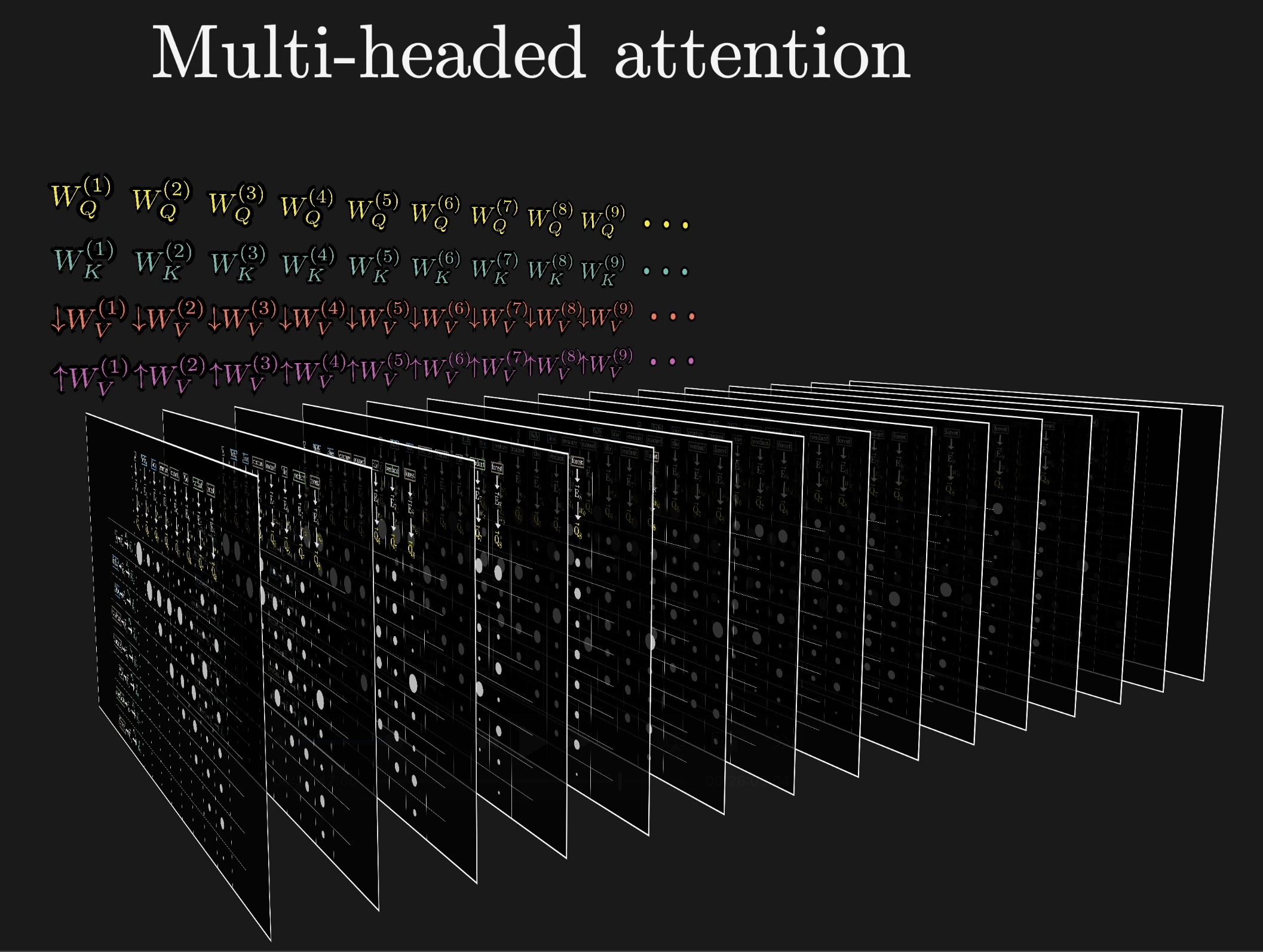
GPT-3, for example, uses 96 attention heads inside each block. Just to spell it all out very explicitly, this means you have 96 distinct key and query matrices producing 96 distinct attention patterns. Then each head has its own distinct value matrices used to produce 96 sequences of value vectors. These value vectors are then all added together using the corresponding attention patterns as weights.
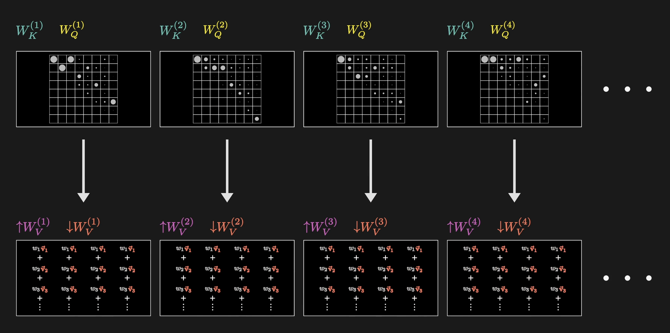
What this means is that for each token, or position in the context, every one of these heads produces a proposed change, labeled as , to be added to the embedding in that position. Then, all of these proposed changes would be added up, one for each head, and the result is added to the original embedding of that position.
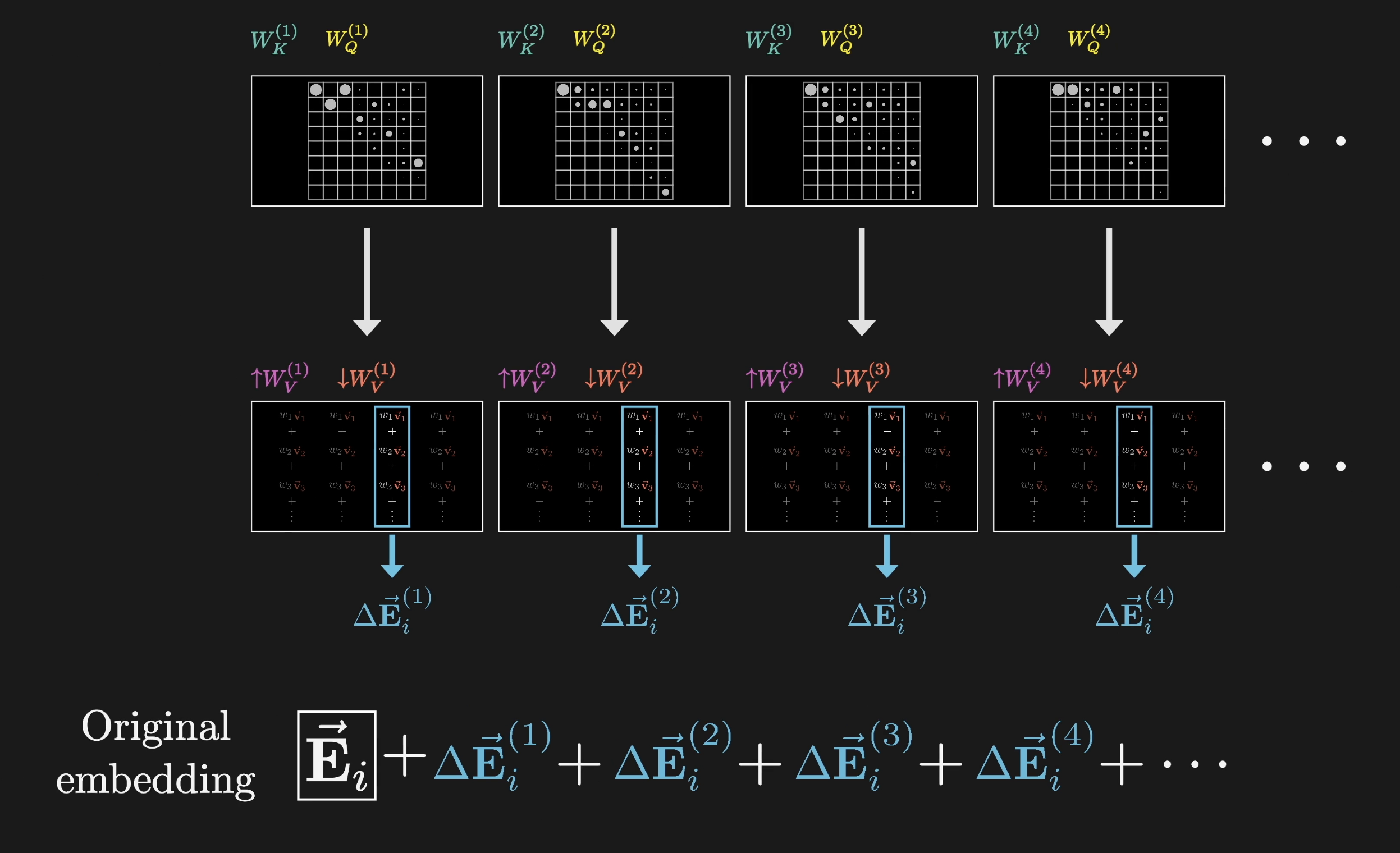
This entire sum would be one slice of what's outputted from this multi-headed attention block; a single one of those refined embeddings that pops out the other end of it.

Again, this is a lot to think about, so don't worry at all if it takes some time to sink in. The overall idea is that by running many distinct heads in parallel, the model is given the capacity to learn many distinct ways that context changes meaning.
Pulling up our running tally for parameter count, with 96 heads-each including its own variation of these four matrices-each block of multi-headed attention ends up with around 600 million parameters.
In the preview from the last chapter, we saw how data flowing through a transformer doesn't just flow through a single attention block. For one thing, the data also flows through these other operations called multi-layer perceptrons, which we'll talk more about in the next chapter.
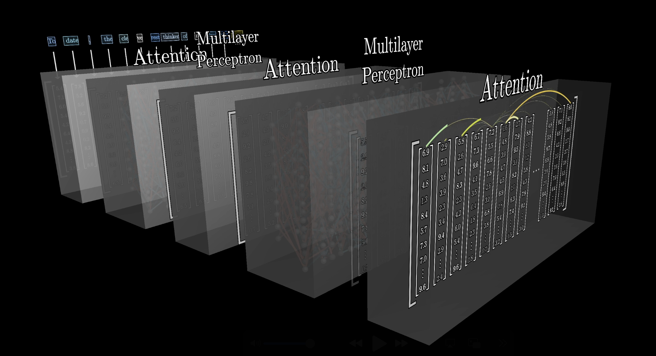
This process is then repeated many, many times as the data goes through many, many copies of both operations.
What this means is that after a given word absorbs some of its context, there are many more chances for this more nuanced embedding to be influenced by its more nuanced surroundings.
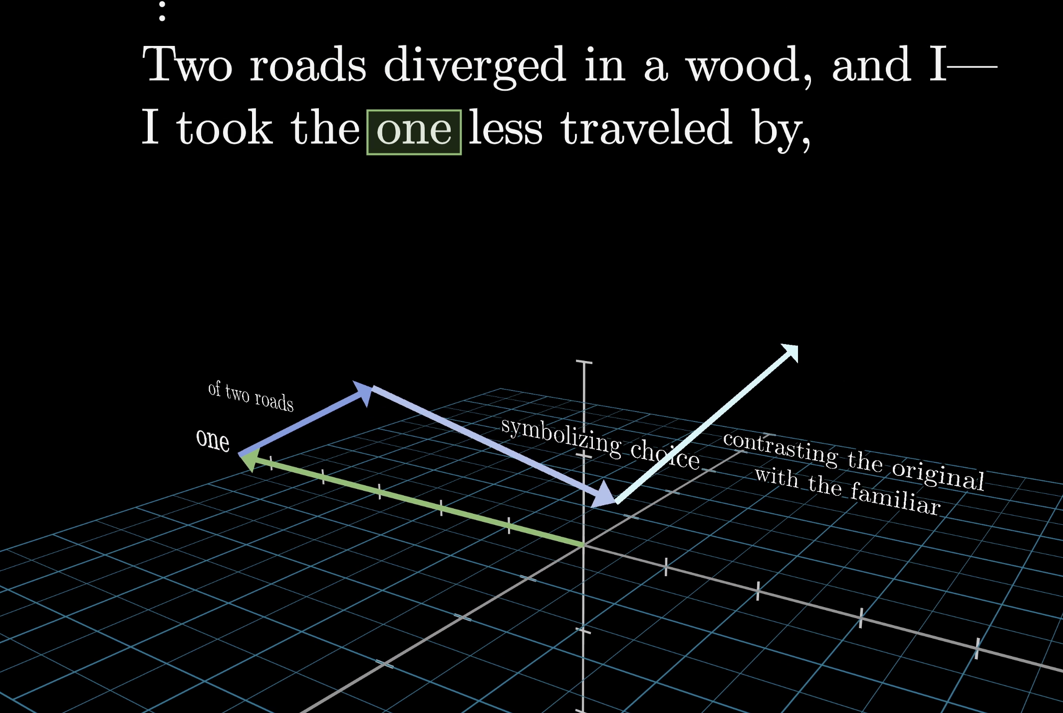
The further down the network we go, with each embedding taking in more and more meaning from all the other embeddings, which themselves are getting more and more nuanced, the hope is that there's the capacity to encode higher-level and more abstract ideas about a given input beyond just descriptors and grammatical structure-things like sentiment, tone, and whether it's a poem and things like that.
Going back once more to our parameter counting, GPT-3 includes 96 distinct layers, bringing the total number of key, query, and value parameters to just under 58 billion, all devoted to the attention heads. That is a lot, but it's only about a third of the billion that are in the network in total. So even though attention gets all of the attention, the majority of parameters come from the blocks sitting in between these steps.

This is about a third of the total parameters in GPT-3!
In the next chapter, we will talk more about those other blocks, knwown as the multi-layer perceptron, and also a lot more about the training process.
A big part of the story for the success of the attention mechanism is not so much any specific kind of behavior that it enables, but the fact that it's extremely parallelizable, meaning that it can run a huge number of computations in a short time using GPUs. Given that one of the big lessons about deep learning in the last decade or two has been that scale alone seems to give huge qualitative improvements in model performance, there's a huge advantage to parallelizable architectures that allow for scaling.
More Resources
If you want to learn more about this stuff, here are a couple of links.
- Let's build GPT: from scratch, in code, spelled out.
- What does it mean for computers to understand language?
In particular, anything produced by Andrej Karpathy or Chris Ola tend to be pure gold.
In this lesson, we just covered attention in its current form, but if you're curious about more of the history for how we got here and how you might reinvent this idea for yourself, here is a video giving a lot more of that motivation:
Also, Britt Cruz from the channel The Art of the Problem has a really nice video about the history of large language models.
Thanks
Special thanks to those below for supporting the original video behind this post, and to current patrons for funding ongoing projects. If you find these lessons valuable, consider joining.